How can a few streamflow measurements help to predict daily hydrographs at almost ungauged sites?

Figures & data

Table 1 Common signs of correlation between nitrate concentrations [NO₃] in river flows (daily values and time variability) and some hydrological variables: antecedent daily river flow (Q_j–i), daily river flow (Q_j) and baseflow index (BFI). CV: coefficient of variation.

	Qj–i	Qj	BFI
[NO3]j	(+)	(−)
CV [NO3]j			(−)

Fig. 1 Reconstruction and segmentation of a daily hydrograph at an almost ungauged pollution-control site: a contribution to meta-analysis of river quality data sampling. Note that uncertainty bounds should bracket the simulated hydrograph (not shown). Segmentation was performed according to the procedure described in the section “Comparative Assessment”.

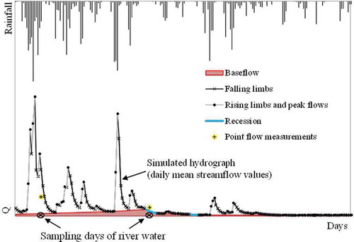
Fig. 2 Location of the 149 streamgauges and the 21 catchments of pollution-control sites used in this study.

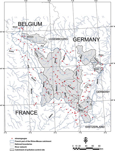
Table 2 Main characteristics of the 21 French pollution-control sites used in this study. See Fig. 1 for locations.

No.	Code	Rivers and pollution-control sites	Area (km^2)	No. of point flow measurements (1971–2010)	Closest basin with continuous streamgauge stations (for cross-validation)	Distance from pollution-control site (km)
1	2094900	Moselle@Sierck	11 470	270	Moselle@Perl	0.4
2	2005700	Doller@Reiningue	187	156	Doller@Reiningue	0.0
3	2018500	Ill@Colmar	1833	72	Ill@Colmar	0.7
4	2018500	Thur@Stattfelden	257	155	Thur@Pulversheim	0.2
5	2028000	Andlau@andlau	37	144	Andlau@andlau	0.8
6	2030200	Ehn@Meistratzheim	60	82	Ehn@niedernai	0.9
7	2046000	Sauer@Beinheim	522	286	Sauer@Beinheim	0.5
8	2047500	Lauter@Wissembourg	272	144	Lauter@Wissembourg	0.0
9	2049900	Cleurie@cleurie	58	150	Cleurie@cleurie	0.6
10	2051600	Neune@Laveline-devant-Bruyère	95	142	Neune@Laveline-devant-Bruyères	0.0
11	2057250	Madon@Mattaincourt	371	11	Madon@Mirecourt	0.4
12	2061500	Meurthe@Fraize	73	156	Meurthe@Fraize	0.7
13	2070250	Meurthe@Damelevières	2286	129	Meurthe@Damelevières	0.1
14	2096900	Sarre@Keskastel	878	282	Sarre@Keskastel	0.0
15	2099800	Blies@Blies-Guersviller	1877	66	Blies@Bliesbruck	0.0
16	2106600	Meuse@Goncourt	374	159	Meuse@Goncourt	0.0
17	2106900	Vair@Soulosse-sous-saint-Elophe	447	140	Vair@Soulosse-sous-saint-Elophe	0.0
18	2109000	Meuse@Saint-Mihiel	2547	188	Meuse@Saint-Mihiel	0.0
19	2115775	Ton@Ecouviez	305	144	Ton@Ecouviez	0.0
20	2115900	Loison@Han-les-Juvigny	346	144	Loison@Han-les-Juvigny	0.0
21	2120000	Semoy@Haulme	1337	224	Semoy@Haulme	0.0

Fig. 3 (a) Experimental (dots) and fitted variograms (solid line) used to model the spatial structure of Pearson’s r correlation coefficient for three representative streamgauges. (b) Observed and estimated correlations resulting from a leave‐one‐out cross‐validation of the respective variograms.

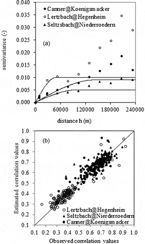
Fig. 4 Map showing the spatial distribution (ordinary kriging) of Pearson’s r values estimated between the daily streamflow time series at the Koenigsmacker streamgauge (Canner River) and all other streamgauges (•) in the study area. In the basic MC method, allowing only a single-best neighbour, the Koenigsmaker streamgauge would be used as a reference streamgauge for the Perl pollution-control site (▼) located on the Mosel River. Contours of the Canner@Koenigsmacker and Mosel@Perl catchments are also shown.

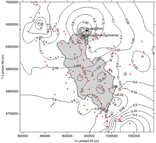
Fig. 5 Changes in mean and percentiles (10% and 90%) for the performance of the MC method according to the number of neighbour catchments,for the 21 French pollution-control sites used (1990–2009).

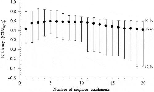
Fig. 6 Example (of the Lauter@Wissembourg catchment) of random streamflow data sampling for selecting the neighbour catchments (DISP and Q–Q methods), n = 30 d. Dots (○) are used for computing the error metric defined in equation (3). Note that point flow measurements were stopped after 2002.

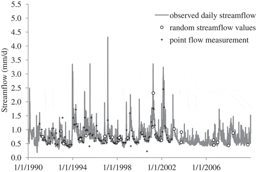
Fig. 7 Impact of the size of daily flow samples (n) and the number of NCs on the efficiency of the Q–Q method. Results are given for the 21 French pollution-control sites used in this study and the period 1990–2009.

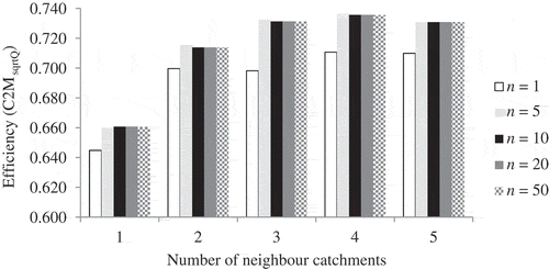
Table 3 Impact of the number n of streamflow values sampled from the daily observed hydrographs on the efficiency (C2M_√Q) of the Q–Q method (option allowing four neighbours). Results are given for the 21 French pollution-control sites used in this study and the period 1990–2009.

Statistics	Number of streamflow values (n)*
	1	5	10	20	50
Minimum	0.340	0.354	0.435	0.435	0.435
Maximum	0.946	0.959	0.970	0.970	0.970
1st quartile (25%)	0.593	0.602	0.596	0.596	0.596
Median (50%)	0.717	0.767	0.766	0.766	0.766
3rd quartile (75%)	0.869	0.878	0.878	0.878	0.878
Mean	0.712	0.736	0.736	0.736	0.736

*sampling is repeated 100 times.

Fig. 8 Comparison of efficiency for the four tested distance-based regionalization methods for the 21 French pollution-control sites used, 1990–2009. MC: map correlation method (option allowing five neighbours); SP: spatial proximity (output averaging); DISP: discrete parameterization of the GR4J rainfall–runoff model at the site of interest (option allowing four neighbours, n = 30 d, α = 0); Q–Q: streamflow–streamflow method (option allowing four neighbours, n = 10 d).

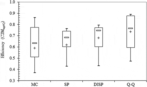
Table 4 Contingency table of days classified for different parts of the hydrograph. Results are given for the daily observed and simulated (Q–Q method) hydrographs of the River Mosel at Perl (11522 km²) for the period 1990–2009. Q–Q: streamflow-streamflow method (option allowing four neighbours, n = 10 days).

	Simulated hydrograph				Total
	Days classified as…	Rising limb*	Falling limb	Recession (Baseflows)
	Rising limb*	2069	661	24	2754
Observed	Falling limb	636	3702	79	4417
hydrograph	Recession	6	11	117	134
	Total	2711	4374	220	7305

*including peak flows.

Fig. 9 Comparison of agreement for the four tested distance-based regionalization methods for the 21 French pollution-control sites used, 1990–2009: (a) rising limbs; (b) falling limbs; (c) recession (baseflows). See Fig. 8 for legend.

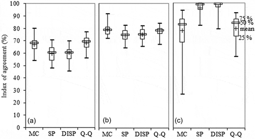
Fig. 10 Maps showing the neighbour catchment(s) (in grey) for the target catchment of the Doller@Reiningue (▼), 187 km². (a) MC method; (b) SP method; (c) streamflow–streamflow method; and (d) DISP method. The four neighbours whose model parameters occur in more than half of the 100 simulations of n are indicated by white circles.

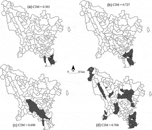
Fig. 11 Comparison between point flow measurements and daily streamflow values. (a) Mosel@Sierck (pollution-control site) vs Mosel@Perl (streamgauge station): 270 days; the mean annual streamflow is close to 145 m³/s. (b) Meurthe@Fraize: 156 days; the mean annual streamflow is close to 2 m³/s. Measurement period refers to 1990–2005 in both cases.

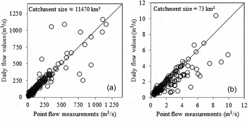
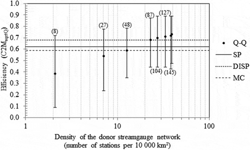
Fig. 12 Changes in mean and percentiles (10% and 90%) for the performance of the Q–Q method according to the reduction of the density of the donor streamgauge network for the 21 French pollution-control sites used, 1990–2009. Horizontal lines provide the mean efficiency of each of the three other regionalization methods considering the full (i.e. existing) donor streamgauge network, with the number of donor catchments for the current density level in parentheses. See Fig. 8 for legend.