Hybrid method to update the design flood shape for spillway operation in a dam: case study of the Huites Dam, Mexico

Figures & data

Figure 1. Hybrid method blocks diagram.

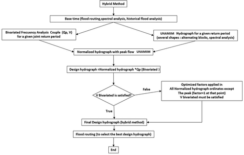
Figure 2. Ramírez and Aldama joint return period.

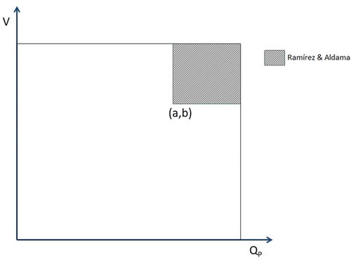
Figure 3. Huites Dam location on the Fuerte River, Sinaloa, México. Source: Institute of Engineering, UNAM.

Institute of Engineering, UNAM.

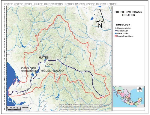
Table 1. Parameters of better adjustment for the double Gumbel pdf for the maximum discharge Q_p and volume V at Huites Dam, Sinaloa, México.

Parameter	Qp	V
α1	0.00117	0.00191
β1	1454.89	1068.72
α2	0.0005900	0.0010190
β2	7496.34	3644.45
P	0.925	0.955
Error	199.01	67 897

The parameter equivalences indicated with the marginal parameter functions (Equations (3) and (4)) are: for Q_p: α₁ = 1/c₁, β₁ = – α₁, α₂ = 1/c₂ and β₂ = – α₂; and for V: α₁ = 1/c₃, β₁ = – α₃, α₂ = 1/c₄ and β₂ = – α₄.

Figure 4. Results of adjusting the double Gumbel function to the annual maximum mean daily flow Q_p for Huites Dam, Sinaloa, México.

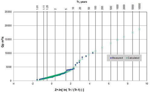
Figure 5. Variation of the double Gumbel function parameters with the duration for the maximum average flows – study of Huites Dam, Sinaloa, México.

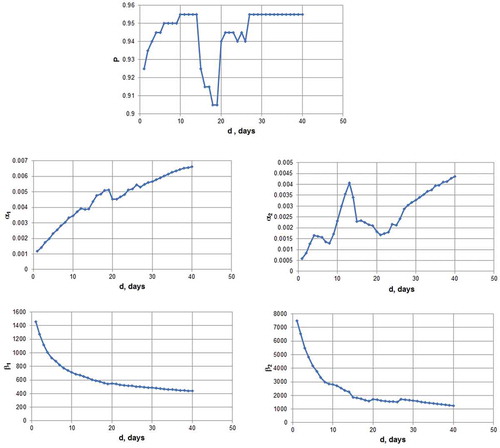
Figure 6. Flow–duration–return period curves by the UNAMIIM approach.

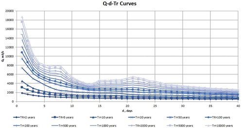
Figure 7. Design flood for T_r= 10 000 years based on UNAMIIM alternating blocks, for Huites Dam, Sinaloa, México.

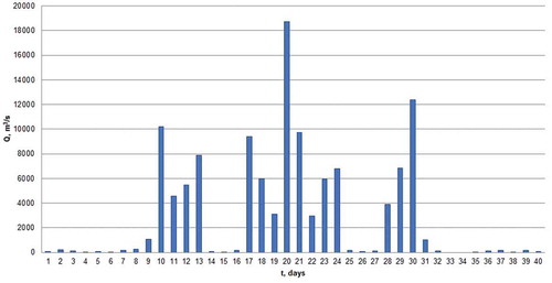
Figure 8. Results of adjusting the double Gumbel function to the volumes V for Huites Dam, Sinaloa, México.

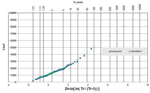
Table 2. Search interval of the parameters of the double Gumbel bivariate distribution function for the genetic algorithm and optimal solution with GA. Huites Dam, Sinaloa, México.

	Lower limit	Marginals Qp and V	Upper limit	GA
Qp parameters
a1	–3000	–1454.9	–500	–1275.6279
c1	400	854	1000	568.38893
a2	–9000	–7496.3	–2000	–3674.0013
c2	1000	1694.9	4000	1864.2842
PQ	0.5	0.9250	0.99	0.74571032
V parameters
a3	–3000	–1068.7	–10	–1001.6175
c3	80	523	900	480.57802
a4	–5500	–3644.5	–500	–1686.2545
c4	50	981.4	1200	791.72491
PV	0.5	0.9550	0.99	0.78323008
m	1.1	1.4617	2.5	1.3419996

Figure 9. Comparison of empirical and calculated double Gumbel bivariate distribution function with respect to an identity function.

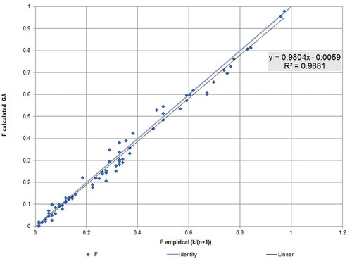
Figure 10. Volume–peak joint return period curves by bivariate analysis for the Huites Dam, Sinaloa, México.

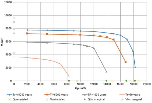
Table 3. Parameters of double Gumbel marginal functions from bivariate analysis.

Parameter	Qp	V
α1	0.001658	0.0169
β1	1319.4	62.644
α2	0.000550845	0.003244611
β2	3674.856	403.336
P	0.789	0.514

The parameter equivalences indicated with the marginal parameter functions (Equations (3) and (4)) are as follows: for Q_p: α₁ = 1/c₁, β₁ = – α₁, α₂ = 1/c₂ and β₂ = – α₂; and for V: α₁ = 1/c₃, β₁ = – α₃, α₂ = 1/c₄ and β₂ = – α₄.

Figure 11. Design floods for T_r = 10 000 years by the hybrid method for Huites Dam, Sinaloa, México.

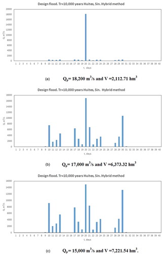
Figure 12. Flood routing results.

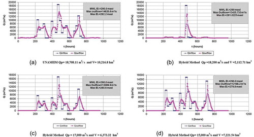
Figure 13. Historical maximum flood routing for Huites Dam.

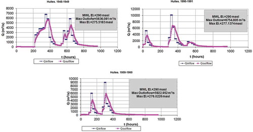
Table 4. Empirical return period for maximum outflow and water level elevation for historical and design floods. Huites Dam, Sinaloa, México.

Maximum flood	Max elevation (masl)	Max ouflow (m^3/s)	Tr (years)
1990–1991	277.14	6754 m^3/s	75
1959–1960	276.02	5923 m^3/s	37.5
1948/49	275.52	5636 m^3/s	25
IIUNAMM	276.77	6499 m^3/s	50
Hybrid method	276.22	6114 m^3/s	50

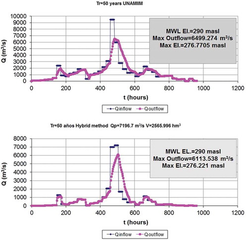
Figure 14. Flood routing T_r = 50 years by UNAMIIM and hybrid methods (Q_p = 7196.7 m³/s and V = 2565.996 hm³).