Capturing flood-risk dynamics with a coupled agent-based and hydraulic modelling framework

Figures & data

Figure 1. Flowchart of the coupled ABMH modelling framework.

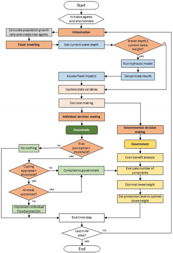
Figure 2. Depth–damage function for protected and non-protected households.

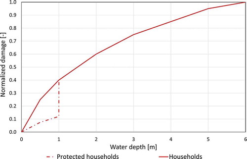
Figure 3. Schematization of the levee geometry.

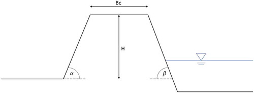
Figure 4. Map of the synthetic case study set-up with the location of the inflow point, levee system, urban centre and households.

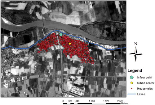
Figure 5. Results of example run with base scenario parameters.

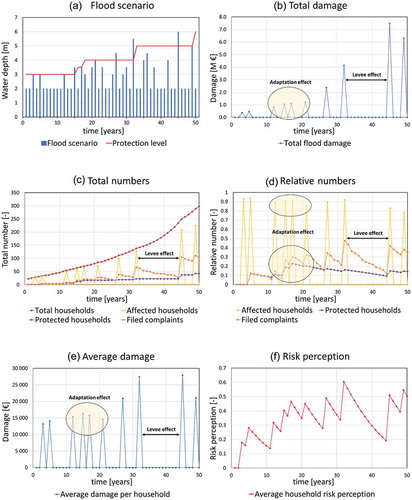
Table 1. Relevant model parameters.

Category	Parameter	Description		Values		Unit
General	$n$	number of simulation years		50		years
Urbanization	$n_{\mathrm{i}\mathrm{n}\mathrm{i}\mathrm{t}}$	initial number of households	10	20	30
	$r_{\mathrm{m}\mathrm{i}\mathrm{n}}$	minimum population growth rate	0.08	0.10	0.12	-
	$r_{\mathrm{m}\mathrm{a}\mathrm{x}}$	maximum population growth rate	0.008	0.010	0.012	-
Decision making	${\mu }_s$	memory decay rate	0.03	0.05	0.07	-
	$\mathrm{R}{\mathrm{P}}_{\mathrm{c}}$	risk perception threshold	0.3	0.5	0.7	-
	$\mathrm{C}{\mathrm{A}}_{\mathrm{c}}$	coping appraisal threshold	0.5	0.7	0.9	-
	$\mathrm{C}{\mathrm{R}}_{\mathrm{m}\mathrm{i}\mathrm{n}}$	minimum complaint rate		0.2		-
	$\mathrm{C}{\mathrm{R}}_{\mathrm{m}\mathrm{a}\mathrm{x}}$	maximum complaint rate		0.8		-
Economic	$c_{\mathrm{a}\mathrm{d}\mathrm{m}}$	administrative cost multiplier	1.3	1.5	1.7	-
	$c_{\mathrm{s}\mathrm{o}\mathrm{i}\mathrm{l}}$	soil cost		30		$\text{euro}/{\mathrm{m}}^3$
	$r$	interest rate		0.05		-
	$k$	time horizon		current time step		years
	$B_c$	crest width		10		m
	$L$	levee length		2000		m
	$\mathrm{t}\mathrm{a}\mathrm{n}\left(\alpha \right)$	angle towards water side		1/4		-
	$tan\left(\beta \right)$	angle towards land side		1/2		-
Hydraulic	$s$	cell size		90 (30)		m
	$n_M$	Manning’s roughness coefficient		0.09		$\mathrm{s}{\mathrm{m}}^{-1/3}$
	$t_{\mathrm{s}\mathrm{i}\mathrm{m}}$	simulation time		40 (144000)		h (s)
	$Q_{\mathrm{i}\mathrm{n},\mathrm{m}\mathrm{a}\mathrm{x}}$	maximum inflow		f(flood scenario, time step)		${\mathrm{m}}^3/\mathrm{s}$
Flood impacts	$d_{\mathrm{m}\mathrm{a}\mathrm{x},r}$	maximum damage per residential building		73879		$\text{euro}/\mathrm{o}\mathrm{b}\mathrm{j}$

Parameters values indicated in bold are those used to run the coupled ABMH modelling framework as benchmark for assessing the influence of stochasticity and model parameters on the model output.

Figure 6. Agent locations in time steps 32 and 44. Protected households are marked by a thicker (blue) outline.

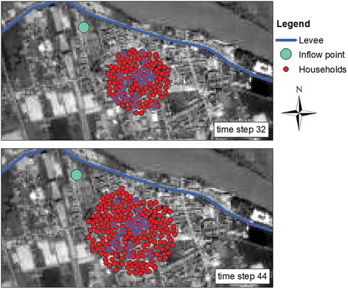
Figure 7. Cost–benefit analyses at four specific time steps during the simulation window. EAD: the expected annual flood damage, ACC: the annual construction cost, and TC: the total cost.

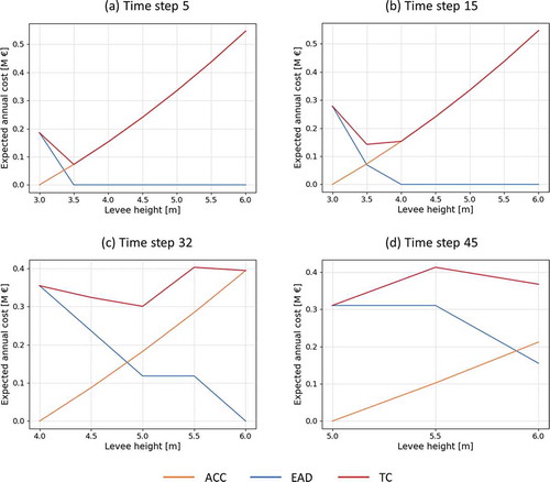
Table 2. Results of sensitivity analysis and relative contribution of model parameters.

Parameter	Value	Number of runs	Average cumulated damage	Relative change	Standard deviation
			(× 10^7 €)	(%)	(× 10^6 €)
Stochasticity	Base scenario	100	2.65	-	1.76
$n_{\mathrm{i}\mathrm{n}\mathrm{i}\mathrm{t}}$	10	50	1.85	–30.3	0.78
	30	50	3.00	+13.3	3.72
$r_{\mathrm{m}\mathrm{a}\mathrm{x}}$	0.08	50	2.23	–15.7	1.10
	0.12	50	2.71	+2.3	3.59
$r_{\mathrm{m}\mathrm{i}\mathrm{n}}$	0.008	50	2.38	–10.0	0.88
	0.012	50	2.86	+7.9	2.09
${\mu }_s$	0.03	50	2.39	–9.8	1.05
	0.07	50	2.81	+6.0	1.92
$c_{\mathrm{a}\mathrm{d}\mathrm{m}}$	1.3	50	2.57	–2.8	3.32
	1.7	50	2.67	+0.6	1.63
$\mathrm{C}{\mathrm{A}}_c$	0.5	50	2.65	± 0.0	1.87
	0.9	50	2.81	+5.9	1.77
$\mathrm{R}{\mathrm{P}}_c$	0.3	50	2.74	+3.5	3.31
	0.7	50	2.59	–2.2	1.08

Bold print indicates the relative change compared to average cumulated damage for the base scenario.

Figure 8. Changes in mean and standard deviation for an increasing number of runs.

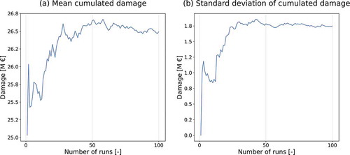
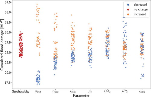
Figure 9. Comparison of the influence of different parameters. Values applied for parameter changes are listed in Table 1.