Suitability of satellite-based hydro-climate variables and machine learning for streamflow modeling at various scale watersheds

Figures & data

Figure 1. Map of the study area showing the Upper Mississippi River Basin (top) and its subwatersheds (bottom left and right). Stars indicate streamflow gauging stations used in this study. Note that the subwatershed downstream of the gauging stations are excluded in the models (shown by lighter colors). The sub-watershed IDs are labelled according to USGS Watershed Boundary Dataset (WBD) Hydrologic Units (HU). USGS gauge numbers are given for the watershed outlets.

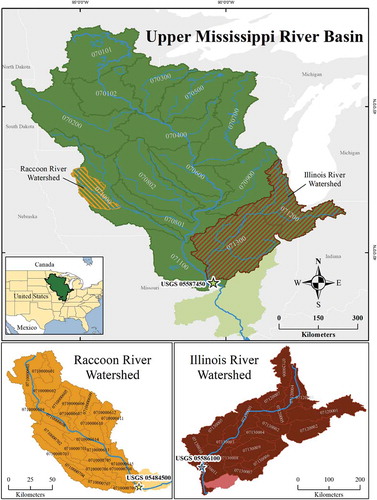
Table 1. Summary of watershed characteristics of the study sites.

Name	HU Code	No. of HUs	Average size of HUs	Modeled area	Avg. LST	Max. LST	Min. LST	Ave precipitation
			(km^2)	(km^2)	(°C)	(°C)	(°C)	(mm/year)
UMRB	6	15	29,851	447 771	8.61	26.14	–16.52	989
IRW	8	18	4,008	72 144	11.66	27.88	–14.82	1086
RRW	10	24	370	8 871	10.44	27.68	–15.00	972.67

UMRB: Upper Mississippi River Basin; IRW: Illinois River Watershed; RRW: Raccoon River Watershed. HU: hydrological unit; LST: land surface temperature.

Figure 2. Summary of data sources and processing applied on the dataset used in the MLM. Processed variables were resampled according to the HUs of each study site.

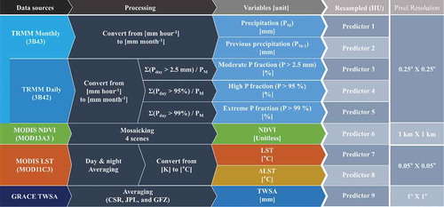
Figure 3. Decision tree processes (a) showing an example of covariant space where Y (predictand or target) is explained by X1 and X2 (predictors). The covariant space can be approximated by rectangular spaces (b) and (c), each representing the first node and entire nodes of the decision tree (d).

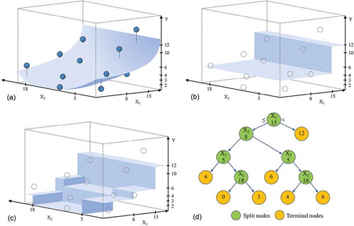
Figure 4. Schematic diagram of the boosting process in the boosted regression tree (BRT) method.

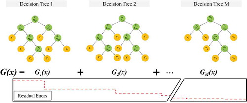
Figure 5. Conceptual diagram of the design of training data.

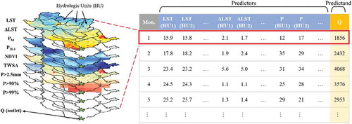
Figure 6. Workflow and data requirements for training and testing in this study.

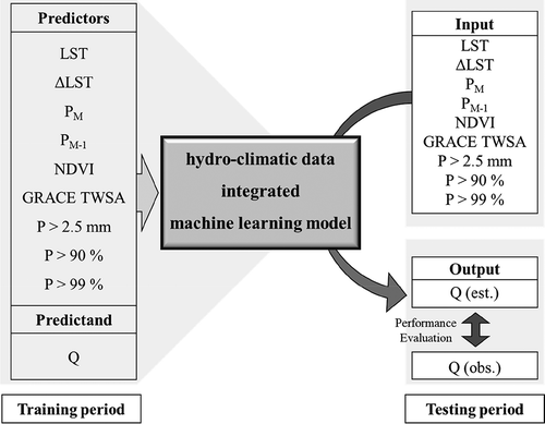
Figure 7. Streamflow model performance according to K-fold numbers.

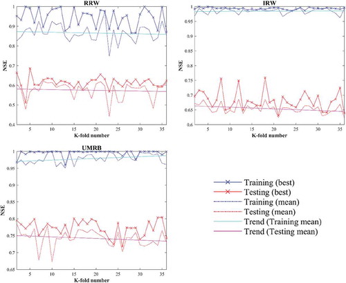
Table 2. Performance metrics for training and testing.

Site	Mean Q (m^3/s)	K-fold	Training				Testing
			NSE	R^2	PBIAS (%)	MAE (m^3/s)	NSE	R^2	PBIAS (%)	MAE (m^3/s)
RRW	71.16	5	0.99	0.99	5.56 × 10^−5	5.48	0.69	0.71	5.81	23.67
IRW	760.60	18	0.98	0.98	1.75 × 10^−4	61.45	0.76	0.80	−10.96	186.28
UMRB	3791.16	35	0.96	0.96	2.05 × 10^−8	383.46	0.80	0.82	−9.28	773.92

NSE: Nash–Sutcliffe efficiency; R2: coefficient of determination; PBIAS: percent bias; MAE: mean absolute error.

Figure 8. Scatterplots of model-simulated vs observed streamflow for training: (a) RRW, (c) IRW, and (e) UMRB; and testing: (b) RRW, (d) IRW, and (f) UMRB.

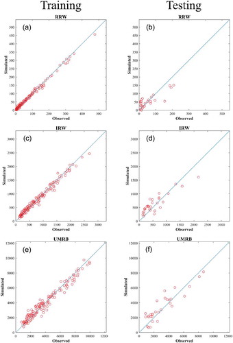
Figure 9. Time series plots of model-simulated streamflow and observed streamflow for the entire study period for (a) UMRB, (b) IRW, and (c) RRW.

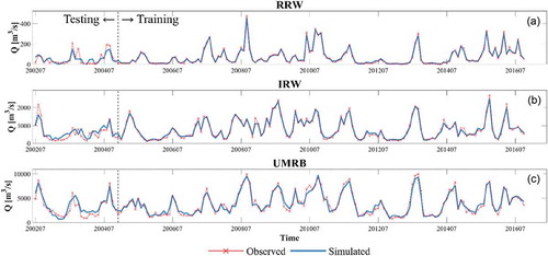
Figure 10. Relative importance of predictor variables for each watershed: (a) RRW, (b) IRW, and (c) UMRB.

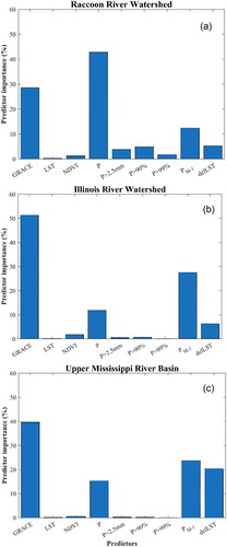
Figure 11. Map showing the relative contribution of sub-watersheds in simulating the MLMs for each watershed. Darker shading shows high relative importance and lighter shading shows low or no importance.

Table 3. Comparison of streamflow estimation performances between existing process-based model results (SWAT) and machine learning modellng (MLM) for each study site.

Site	Process-based model				MLM (this study)
	Reference	Validation (testing) period	NSE	PBIAS	NSE	PBIAS
RRW	Jha et al. (2007)	1993–2003	0.88	-	0.69	5.81%
IRW	Yen et al. (2016)	1990–2001	0.72	13.91%	0.76	–10.96%
UMRB	Jha et al. (2006)	1988–1997	0.81	3.9%	0.80	–9.28%

Note: The testing period for the MLM is 2002–2004. RRW: Raccoon River Watershed; IRW: Illinois River Watershed; UMRB: Upper Mississippi River Basin. NSE: Nash–Sutcliffe efficiency; PBIAS: percent bias.

Jha, M.K., Gassman, P.W., and Arnold, J.G., 2007. Water quality modeling for the Raccoon River watershed using SWAT. Transactions of the ASABE, 50 (2), 479–493.

 Web of Science ®Google Scholar

Yen, H., et al. 2016. Application of large-scale, multi-resolution watershed modeling framework using the Hydrologic and Water Quality System (HAWQS). Water, 8 (4), 164. doi:10.3390/w8040164

 Web of Science ®Google Scholar

Jha, M., et al. 2006. Climate change sensitivity assessment on Upper Mississippi River Basin streamflows using SWAT 1. JAWRA Journal of the American Water Resources Association, 42 (4), 997–1015. doi:10.1111/j.1752-1688.2006.tb04510.x

 Web of Science ®Google Scholar