Discharge estimation for medium-sized river using multi-temporal remote sensing data: a case study in Brazil

Figures & data

Table 1. Hydrological variables inferred from satellite images planimetric properties. ACC: accuracy; RMSE: root mean square error; RRMSE: relative root mean square error (divided by mean of observations); r2: coefficient of determination; $y_i$: predicted value, $x_i$: observed value

Estimated variable	Mission	Results	References
Water surface	SPOT Vegetation	ACC = 95.4%	Haas et al. (2009)
	Landsat	ACC = 97%	Mueller et al. (2016)
	Landsat	ACC = 99.2%	Pekel et al. (2016)
Discharge	ERS 1	r2 = 0.83	Smith et al. (1996)
	Quickbird-2	ACC = 97%	Xu et al. (2004)
	Quickbird-2	ACC = 80%	Zhang et al. (2004)
	MODIS	r2 = 0.81	Smith and Pavelsky (2008)
	Landsat	RRMSE 26–41%	Gleason et al. (2014; 2014)
	MODIS	RMSE = 10%	Elmi et al. (2015)
Propagation speed	MODIS	$y_i$ = 1.01 m/s $x_i$ = 0.97 m/s	Smith and Pavelsky (2008)
	MODIS	-	Sichangi et al. (2018)

Figure 1. Location of the São Francisco River reach used as test area showing the in situ hydrological stations (left) and geographical context in the South American continent (right)

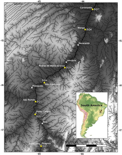
Table 2. Station location

Station location	ANA code	Code	S Latitude/W Longitude	Mean discharge (m^3/s)	Drainage area (km^2)	Altitude (m a.s.l.)
Pirapora	41135000	${\mathrm{S}}_{Q1}$	17°22ʹ9.12ʹ’/44°56ʹ35.2ʹ’	841	62200	480
Cachoeira da Manteiga	42210000	${\mathrm{S}}_{Q2}$	16°39ʹ 25.92ʹ’/45°4ʹ50.9ʹ’	1169	107000	467
São Romão	43200000	${\mathrm{S}}_{Q3}$	16°22ʹ21.00ʹ’/45°4ʹ12.0ʹ’	1569	154000	464
São Francisco	44200000	${\mathrm{S}}_{Q4}$	15°56ʹ57.84ʹ’/44°52ʹ4.1ʹ’	1808	184000	457
Pedras de Maria da Cruz	44290002	${\mathrm{S}}_{Q5}$	15°36ʹ3.96ʹ’/44°23ʹ48.1ʹ’	2017	194000	451
Manga	44500000	${\mathrm{S}}_{Q6}$	14°45ʹ25.92ʹ’/43°55ʹ55.9ʹ’	1953	202000	440
Carinhanha	45298000	${\mathrm{S}}_{Q7}$	14°18ʹ15.84ʹ’/43°45ʹ47.9ʹ’	2192	254000	427

Figure 2. Steps for measuring width. Background: S1 Image; VV; acquisition 08/03/2016

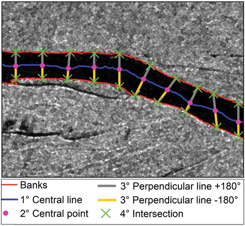
Figure 3. Illustration of the extraction of the river width from a classified image

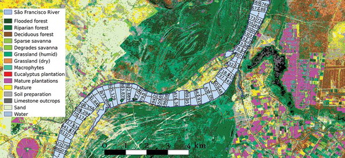
Figure 4. K-fold cross-validation example for k = 5. Light grey: training data, Dark grey: test data. The method first divides the data set in k subsets, then uses k – 1 subsets for training while keeping the remaining one for validation. k iterations are performed, each one testing a model build from a different fold generating a validation estimate. The mean absolute error (MAE) was used here

Figure 5. The three different methods of virtual (width) stations definitions: (a) individual width ($w$) at-a-station, (b) systematic average width stations ($w_n$) calculated for the whole river reach every 10 km and (c) selected average width stations ($w_s$) defined by statistically selecting river sections with the most width variations

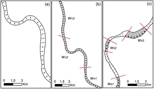
Figure 6. Illustration of the set of 952 river cross-sections widths organized by quartiles (25% = 55.5 m, 50% = 90.62 m, 75% = 228.86 m)

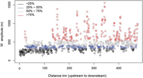
Table 3. Transferred discharge (QWQ) of station SQ3 to a virtual station 64 km downstream that coincides with station SQ4. The PFE gives an idea of the errors generated by the approach

Dates 1–2	Station SQ3 (m^3/s)	Station SQ4 (m^3/s)	QWQ (m^3/s)	PFE QWQ – SQ4 (%)
01–02/03/2016	596.9	658.0	713.2	8.39
08–09/03/2016	909.4	1061.7	1086.5	2.34
03–04/12/2016	685.2	832.6	818.7	–1.67
15–16/12/2016	2169.6	2407.2	2592.3	7.69
13–14/02/2017	1297.0	1661.5	1549.7	–6.73
09–10/03/2017	549.9	630.7	657.1	4.18
13–14/11/2017	559.2	815.0	668.1	–18.02
10–11/12/2017	1751.3	2059.0	2092.5	1.63
28–29/12/2017	426.6	547.5	509.7	–6.90
15–16/01/2018	545.3	678.7	651.5	–4.01
20–21/02/2018	491.2	698.3	586.8	–15.97
16–17/03/2018	1715.0	1934.8	2049.1	5.91
21–22/04/2018	439.2	570.2	524.8	–7.96
07–08/05/2018	294.0	335.1	351.2	4.81
17–18/05/2018	312.3	333.2	373.1	11.96
06–07/06/2018	357.9	383.1	427.6	11.63
21–22/06/2018	338.6	348.3	404.5	16.15
16–17/07/2018	357.9	363.6	427.6	17.60
14–15/08/2018	385.6	387.0	460.7	19.05

Figure 7. Transferred discharge data (SQ QWQ) of station S_Q3 to a point 64 km downstream that coincides with station S_Q4.

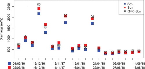
Figure 8. Model performance evaluation for virtual stations generated from the three methods

Figure 9. Evaluation metrics used to compare the results from the three discharge estimation methods: (a) individual width, $w$; (b) systematic average, $w_n$ and (c) selected average, $w_s$

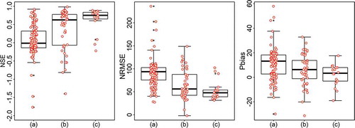
Figure 10. The best curves for the $w-Q$ relationship by method and the respective analysis sections in the river

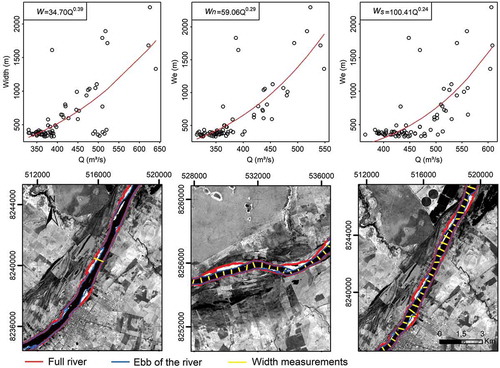
Table 4. Best fit power functions achieved by each method

Method	Equation	NSE	NRMSE	Pbias
$w$	$Q={\left(\frac{W}{34.70}\right)}^{\frac{1}{0.39}}$	0.92	27.42	5.1
$w_n$	$Q={\left(\frac{We}{59.06}\right)}^{\frac{1}{0.29}}$	0.89	31.5	6.0
$w_s$	$Q={\left(\frac{We}{100.41}\right)}^{\frac{1}{0.24}}$	0.87	34.82	2.8

Table 5. Models $w_s$ method. Bold values indicate best model results

Virtual station	a	b	NSE	NRMSE	Pbias
$w$s1	4.968	0.662	0.760	47.2	2.8
$w$s2	8.358	0.635	0.686	54.0	3,9
$w$s3	70.446	0.296	0.856	36.6	–3.1
$w$s4	100.417	0.243	0.869	34.8	–3.0
$w$s5	56.224	0.313	0.835	39.1	9.5
$w$s6	3.839	0.709	0.706	52.2	5.9
$w$s7	87.266	0.237	0.746	48.6	–1.6
$w$s8	129.009	0.236	0.795	43.6	2.7
$w$s9	80.714	0.297	0.605	60.2	–9.3
$w$s10	10.870	0.582	0.849	37.2	–4.8
$w$s11	0.284	1.083	–0.044	94.6	17.6
$w$s12	263.828	0.109	–0.222	102.3	–19.0
$w$s13	40.654	0.376	0.652	53.8	8.0

Figure 11. Location of the 13 virtual $w_s$ stations

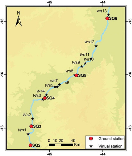
Figure 12. Daily in situ discharge (Q_obs) data (line) compared with estimated discharge calculated from the $w_s$ method for the period March 2016–August 2018

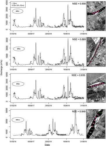
Figure 13. Cross-sections at six locations along this river reach $w_{s4}$

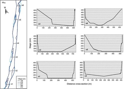
Figure 14. Relationships between (a) exponent $b$ and width amplitude, and (b) NRMSE and width amplitude

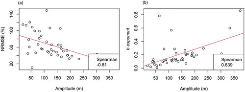
Figure A1. Top Sentinel-1B SAR image of the Pampulha Reservoirs complex. Bottom: difference maps between the SAR image classification results and the precise delineation. Grey pixels represent false negative errors (omitted pixels) and black pixels represent false positive errors (falsely included pixels). Reproduced with permission from the authors

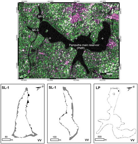
Figure A2. Left: PlanetScope false colour image. Right: water surfaces extracted from Lansat-8, Sentinel-1 and Sentinel-2 images. The background cyan colour shows the reference surface from the Planet Scope image used for determination of accuracy. Reproduced with authorization from the authors

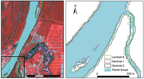
Table A1. List of images acquired with some of their specification and the associated water stage level

Sensor	Image date	Pixel size (m)	Stage (cm)*	Product level
Sentinel-1 (S-1)	15/01/18	10	223.5	Level-1GRD
Sentinel-2 (S-2)	17/01/18	10	217	1 C
PlanetScope	17/01/18	3	217	3A
Landsat/OLI (L-8)	18/01/18	30	213	L1

Table A2. Water surface classification accuracy by sensor, spectral bands and polarizations

Rank	Bands L8	Accuracy L8	Bands S-2	Accuracy S-2	Pol band S-1	Accuracy S-1
1	6	86.43	8,12	94.70	VV	93.79
2	3,6	86.22	3,8	94.48	VH	84.97
3	3,7	86.09	8A,11	94.41	VV+VH	82.00
4	6,7	85.92	8,11	94.32
5	3,6,7	85.88	6,8A,11	94.28
6	3,4,6	85.73	8,11,12	94.25
7	7	85.59	11,12	94.24
8	3,4,6,7	85.53	8A,11,12	94.21
9	3,4,7	85.46	6,8A,11,12	94.16
10	4,6,7	85.28	6,11,12	94.13

Haas, E.M., Bartholomé, E., and Combal, B., 2009. Time series analysis of optical remote sensing data for the mapping of temporary surface water bodies in sub-Saharan western Africa. Journal of Hydrology, 370 (1–4), 52–63. doi:10.1016/j.jhydrol.2009.02.052

 Web of Science ®Google Scholar

Mueller, N., et al., 2016. Water observations from space: mapping surface water from 25 years of Landsat imagery across Australia. Remote Sensing of Environment, 174, 341–352. doi:10.1016/j.rse.2015.11.003

 Web of Science ®Google Scholar

Pekel, J.F., et al., 2016. High-resolution mapping of global surface water and its long-term changes. Nature, 540 (7633), 418–422. doi:10.1038/nature20584

 PubMed Web of Science ®Google Scholar

Smith, L.C., et al., 1996. Estimation of discharge from braid rivers using synthetic apertureradar imagery: potential application to ungauged basins. Water Resources Research, 32 (7), 2021–2034. doi:10.1029/96WR00752

 Web of Science ®Google Scholar

Xu, K., et al., 2004. Estimating river discharge from very high‐resolution satellite data: a case study in the Yangtze River, China. Hydrological Processes, 18 (10), 1927–1939. doi:10.1002/hyp.1458

 Web of Science ®Google Scholar

Zhang, J., et al., 2004. Estimation of river discharge from non-trapezoidal open channel using QuickBird-2 satellite imagery. Hydrological Sciences Journal, 49 (2). doi:10.1623/hysj.49.2.247.34831

 Web of Science ®Google Scholar

Smith, L.C. and Pavelsky, T.M., 2008. Estimation of river discharge, propagation speed, and hydraulic geometry from space: Lena River, Siberia. Water Resources Research, 44 (3). doi:10.1029/2007WR006133

 Web of Science ®Google Scholar

Gleason, C.J., Smith, L.C., and Lee, J., 2014. Retrieval of river discharge solely from satellite imagery and at-many-stations hydraulic geometry: sensitivity to river form and optimization parameters. Water Resources Research, 50 (12), 9604–9619. doi:10.1002/2014WR016109

 Web of Science ®Google Scholar

Gleason, C.J. and Smith, L.C., 2014. Toward global mapping of river discharge using satellite images and at-many-stations hydraulic geometry. Proceedings of the National Academy of Sciences, 111 (13), 4788–4791. doi:10.1073/pnas.1317606111

 PubMed Web of Science ®Google Scholar

Elmi, O., Tourian, M.J., and Sneeuw, N., 2015. River discharge estimation using channel width from satellite imagery. In: 2015 IEEE International Geoscience and Remote Sensing Symposium (IGARSS). Milan: IEEE, 727–730.

 Google Scholar

Sichangi, A., Wang, L., and Hu, Z., 2018. Estimation of river discharge solely from remote-sensing derived data: an initial study over the Yangtze river. Remote Sensing, 10 (9), 1385. doi:10.3390/rs10091385

 Web of Science ®Google Scholar