Figures & data
Table 1. Distribution of nine hydroclimatic and five morphological characteristics of 229 catchments. P99 is the 99th percentile of daily streamflow
Figure 1. Location of the 229 French catchments selected. The streamflow regimes were determined according to the definition of Sauquet et al. (Citation2008)
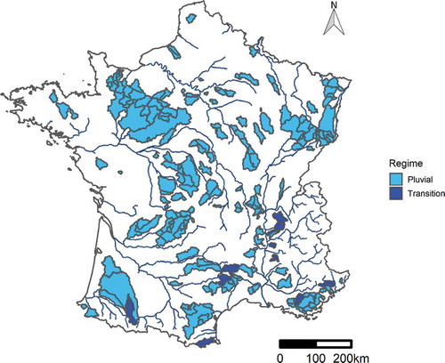
Figure 2. Distribution and localization of the characteristics of 2990 flood events. The distributions are presented between the 5th and 95th percentiles. Parts (b) and (d) present maximum values and part (f) presents mean values. nev is the number of flood events of each season and nc is the related number of catchments
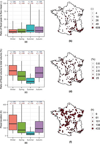
Figure 3. Distribution of catchment seasonal flood volumes compared with seasonal streamflow volume for 2990 flood events in 229 catchments. nev is the number of flood events of each season and nc is the related number of catchments
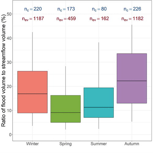
Figure 4. Illustration of the streamflow time windows used to calculate the event bias per catchment and the bias outside periods with events per catchment. The hydrograph presented here corresponds to the Lergue River at Lodève (southern France)
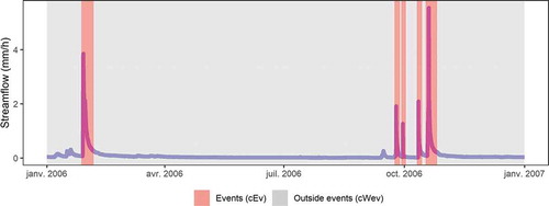
Table 2. Correspondence between bias (β) and bounded bias (βb) values
Table 3. List of the relative characteristics used for the univariate analysis. All characteristics are expressed as percentages
Figure 5. Distribution of GR5H-I performance in calibration and validation periods over 229 French catchments. The distributions are presented between the 5th and 95th percentiles
Figure 6. Difference of (a) cumulative rainfall and KGE; (b) runoff coefficient and KGE in validation mode between P1 and P2
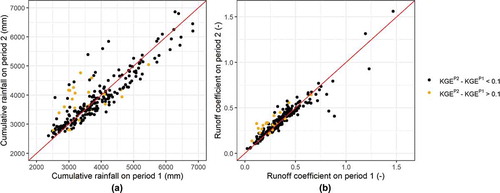
Figure 7. Distribution of GR5H-I bias over 229 catchments and 2990 events. The bias (bounded) was calculated for four levels of hydrograph disaggregation. The distributions are presented between the 5th and 95th percentiles. Calculations were made with cross-validation values, i.e. using simulations on P1 and P2 obtained with the parameter sets optimized on P2 and P1, respectively
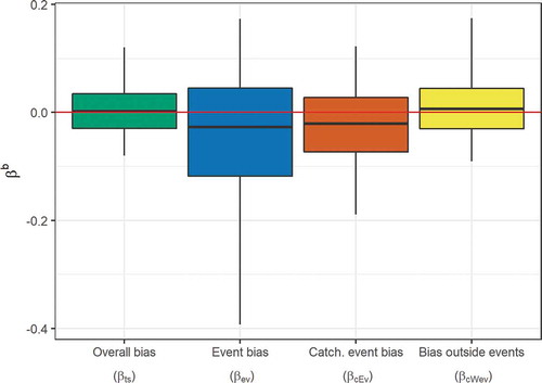
Figure 8. Seasonality of GR5H-I bias over 229 catchments and 2990 events. The bias (bounded) was calculated on four levels of hydrograph disaggregation. The distributions are presented between the 5th and 95th percentiles. Calculations were made with cross-validation values. nc is the related number of catchments and nev is the related number of flood events. Part (c) shows the seasonal distributions for all catchments
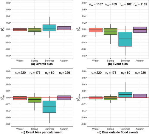
Figure 9. Examples of simulations of summer floods compared with floods that occurred in other seasons. Simulations of GR5H-I are in validation mode. βev is the flood event bias. βts and KGE are the bias and KGE index, respectively, calculated for the entire corresponding validation period
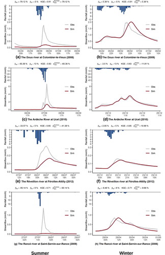
Figure 10. (a) to (e) present the results of a univariate analysis of the relationships between flood characteristics and event bias βevb for 80 catchments in which floods occur in summer. Each characteristic class contains approximatively 211 events. The flood characteristics presented are relative to the mean flood characteristics of the corresponding catchment. (b) is the linear correlation matrix between the relative flood characteristics
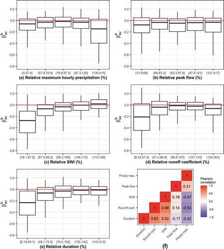
Figure 11. GR5H-I summer event bias per catchment plotted against KGE values for catchments where flood events occurred in summer
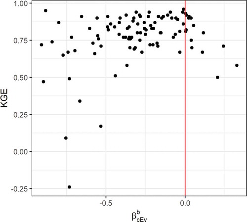
Figure 12. (a) Relationship between GR5H-I simulation of event effective rainfall and event bias (each class contains approximatively 211 events). (b) Relationship between GR5H-I simulation of event effective rainfall and precipitation intensity relative to event duration. The results are for 1054 events that took place in 80 catchments in which floods can occur in summer
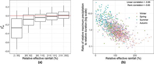
Table A1. List of the variables of GR5H-I expressed for a given time step (mm or mm/h)
Table A2. List of the free parameters of GR5H-I
Figure A1. Diagram of the GR5H-I model (modified from Le Moine Citation2008, Ficchì et al. Citation2019)