Figures & data
Figure 1. (a) The 500-year floodplain of Dresden in Saxony, Germany, with manufacturing and service company premises (as in 2009). (b) Causal loop diagrams of the four socio-hydrological candidate models (model abbreviation in the top right of each box). System variables are represented by words and letters, while internal (solid) and exogenous (dashed) processes are indicated by arcs. Variables and processes that are augmented by the process-oriented loss estimation (blue) and the sector differentiation (orange) are highlighted in colour. The dotted orange arc between and
in the “aug” model does not have a sign as it visualizes the weighting of sector-specific losses according to occupied floodplain area (see section 2.3.2).
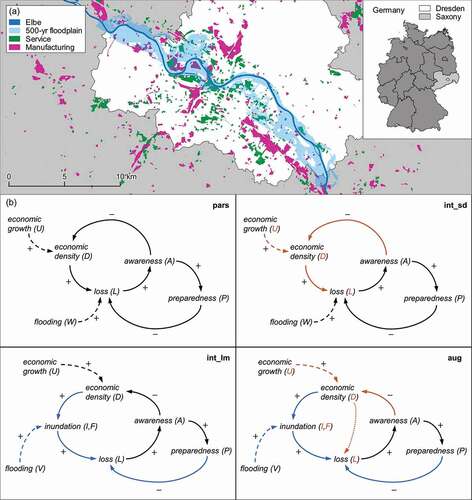
Table 1. Variables and parameters of the socio-hydrological model. The units and
refer to the number of companies in the floodplain and the number of implemented precautionary measures, respectively.
Table 2. Data used for parameter estimation. The temporal coverage indicates for which years of the simulation period the respective data are available.
Figure 2. Fit of the candidate models to data. Each plot panel shows one candidate model: pars, parsimonious; int_lm, intermediate with process-oriented loss estimation; int_sd, intermediate with sector differentiation; aug, fully augmented.
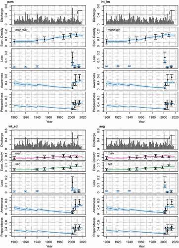
Figure 3. Marginal posterior distributions (log-scale) of the socio-hydrological parameters in the four candidate models: pars, parsimonious; int_lm, intermediate with process-oriented loss estimation; int_sd, intermediate with sector differentiation; aug, fully augmented. The marginal prior distributions are the adopted posterior distributions from Barendrecht et al.’s (2019) model for the residential sector. The points show the median, while the bars correspond to 50% and 95% credible intervals.
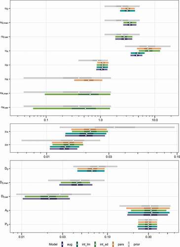
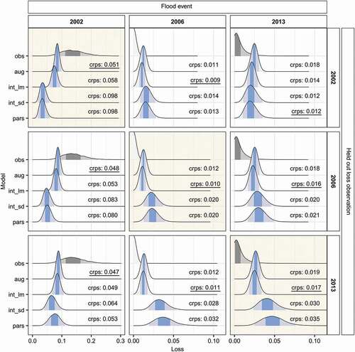
Figure 4. Comparison of modelled and reported flood losses. (a) Aggregated losses for the three observed flood events; (b) sector-specific losses of the 2002 flood. The shaded areas under the curves show 50% and 95% credible intervals. The continuous ranked probability score (crps) quantifies the error of the loss predictions; the best fit is underlined. Model codes: obs, observation; pars, parsimonious; int_lm, intermediate with process-oriented loss estimation; int_sd, intermediate with sector differentiation; aug, fully augmented.
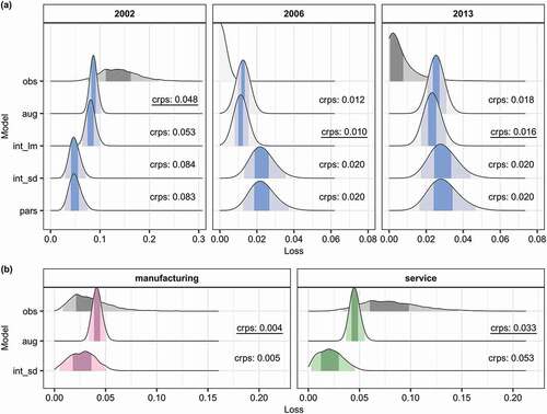
Figure 5. Modelled and observed losses (as in )) for the leave-one-out cross-validation experiment. Panel rows indicate which flood event was held out during model training, while in each column the same loss event is displayed. Plot panels with background shading highlight the predictions for unseen data. Model codes: obs, observation; pars, parsimonious; int_lm, intermediate with process-oriented loss estimation; int_sd, intermediate with sector differentiation; aug, fully augmented.