Figures & data
Figure 1. Schematic representation of systematic change detection in a routing model structure.
Table 1. True parameter formulation for both pre- and post-regulation periods.
Table 2. Detail of scaling factor implementation to capture the future structural changes before and after the river regulation for four plausible scenarios – coefficients of linear () and non-linear (
) models.
Table 3. More detailed description of concepts used in formulating four plausible scenarios.
Figure 2. Normalized innovation sequences for: (a) scenario #1, (b) scenario #2, (c) scenario #3, and (d) scenario #4.
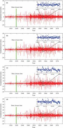
Table 4. Root mean square error under the four devised scenarios.
Figure 3. Visual representation of model performance for the two routing models, the LMM coupled with dual state–parameter updating kernel and LMM without coupling any kernel updating, under scenario #1 (left column) and Scenario #3 (right column) over time.
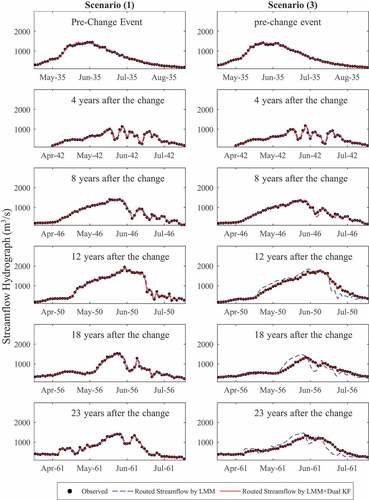
Figure 4. versus
under the four devised scenarios and for the two change criteria: (1) change in the mean (left column) and (2) change in the variance (right column). The points on the convex hull (blue line) are shown with blue squares and the others are shown with red triangles.
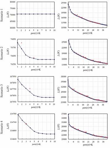
Table 5. Variations of normalized contrast value and the second-order derivative against the number of segments for both the mean and variance measures.
Table 6. Number and location of detected change points based on change in the mean and variance for four devised scenarios.
Figure 5. The pathway of structural evolution for the four devised scenarios along with the change points detected based on the two change criteria: (1) change in the mean (left column) and (2) change in the variance (right column).
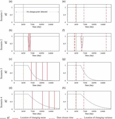
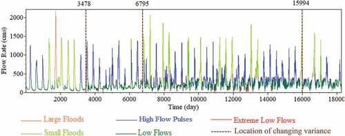
Figure 6. Temporal variability of environmental flow components along with the locations of change points in the variance for scenario #1.