Improving the representation of groundwater processes in a large-scale water resources model

Figures & data

Figure 1. Map of the Cauvery River basin with key features labelled and location inset. Gauging stations are numbered for clarity; corresponding names can be found in Appendix B (Table B1).

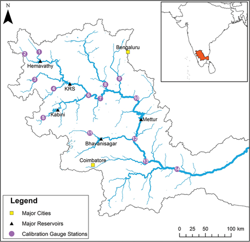
Figure 2. Specific yield values at each layer for the different geological domains. Orange lines denote groundwater abstraction limit.

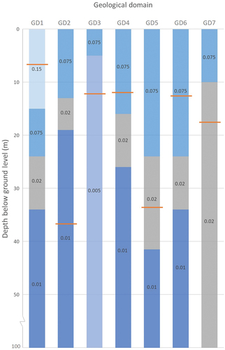
Figure 3. Hydrogeological domains defined for the conceptual groundwater model in GWAVA-GW. For details see Fig. 2.

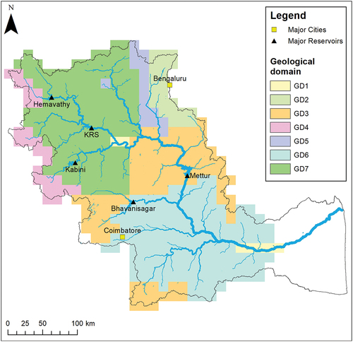
Table 1. Kling-Gupta efficiency (KGE) values for calibration and validation runs at each sub-catchment, for Global Water AVailability Assessment (GWAVA) and GWAVA with improved groundwater scheme (GWAVA-GW), and change in model skill (Δ skill) between the two model versions for calibration and validation (Equation 3(3) $\mathrm{\Delta }\mathrm{s}\mathrm{k}\mathrm{i}\mathrm{l}\mathrm{l}=\frac{\left(KG{E}^{GW}-KGE\right)}{\left(KG{E}^{optimal}-KGE\right)},$(3) ).

Sub-catchment	Calibration			Validation
	GWAVA	GWAVA-GW	Δ skill	GWAVA	GWAVA-GW	Δ skill
1. Thimmanahalli	0.37	0.65	0.44	−0.01	0.53	0.54
2. Sakleshpur	0.25	0.32	0.09	0.02	0.09	0.06
3. Kudige	0.15	0.31	0.19	0.45	0.54	0.17
4. K. M. Vadi	−0.12	−0.01	0.10	−0.05	0.06	0.10
5. Munthankera	0.48	0.64	0.31	0.54	0.70	0.35
6. T. Narasipur	0.60	0.72	0.31	0.11	0.33	0.25
7. Kollegal	0.42	0.59	0.30	0.30	0.36	0.08
8. T. K. Halli	0.38	0.53	0.24	0.59	0.71	0.31
9. T. Bekuppe	−1.07	0.33	0.68	−5.23	−1.87	0.54
10. Biligundulu	0.59	0.65	0.15	0.36	0.26	−0.17
11. Thengumarahada	−0.08	0.49	0.53	−0.10	0.04	0.13

Figure 4. Observed (India-WRIS 2020) and simulated (GWAVA-GW) groundwater levels averaged over time (2007–2014) and over the sub-catchment areas (Fig. 1; Appendix B, Table B1).

Figure 5. Observed and simulated (GWAVA-GW) monthly depth to groundwater, averaged spatially over sub-catchment 2 (Sakleshpur), with the range of observed groundwater depths over the sub-catchment.

Figure 6. Simulated groundwater fluxes averaged over time (2007–2014) and selected sub-catchment areas. Fluxes are grouped as outgoing (abstractions and baseflow) and incoming fluxes (recharge from rainfall, conveyance loss and from lakebeds). Recharge from small-scale interventions is not included as it is negligibly small. For sub-catchment locations and names see Fig. 1 and Appendix B, Table B1.

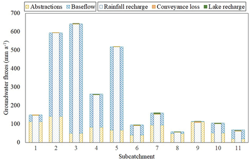
Figure A1. Baseflow and groundwater depths for a test-case single grid cell under artificial drivers: no recharge, constant recharge (at a rate of 2 mm per time step), and variable recharge (grey line, top right plot). Specific yield values are those of the geological domain GD7 (Fig. 2), and the simulations were run with an initial depth of 5 m, h_BF of 18 m, and λ = 0.001 (solid line), 0.002 (dashed line), 0.005 (dotted line), and 0.01 (dot-dash line).

Table B1. Description of selected sub-catchments (Fig. 1) including name of gauging station; modelled area; observed average annual rainfall (1988–2014) (Pai et al. 2014) summed over the sub-catchment area; years used for calibration and validation of both models; and percentage of observed data in the streamflow data used for calibration/validation. Note that climate data used only extended to 2014.

Sub-catchment	Modelled area (km^2)	Precipitation over the sub-catchment (mm a^−1)	Calibration		Validation
			Range	Observed data (%)	Range	Observed data (%)
1. Thimmanahalli	1683	1601	2005–2010	32	2010–2014	82
2. Sakleshpur	748	2514	2006–2011	37	2011–2014	68
3. Kudige	2256	2431	1980–1991	72	2012–2014	78
4. K.M. Vadi	2068	1449	1991–2001	49	2001–2012	71
5. Munthankera	1881	2297	1990–2001	50	2001–2012	69
6. T. Narasipur	14 089	1675	1990–2001	43	2001–2009	62
7. Kollegal	21 040	1448	1990–2001	49	2001–2009	60
8. T. K. Halli	8253	785	1988–1997	50	1999–2001	61
9. T. Bekuppe	4883	836	2008–2012	44	2012–2014	78
10. Biligundulu	40 947	1139	1990–2001	78	2001–2012	78
11. Thengumarahada	1511	1487	1990–2001	55	2001–2004	81
12. Urachikottai	53 407	1105	1990–2001	52	2001–2009	82
13. Kodumudi	56 619	1102	1990–2001	58	2005–2011	81
14. Musiri	80 277	1041	1990–2001	55	2006–2011	78

Table B2. Summary of datasets used to build the model.

Input data	Resolution	Source
GWAVA and GWAVA-GW
Precipitation; maximum and minimum temperatures	0.125°, daily	Indian Meteorological Department (Pai et al. 2014)
Elevation	30 × 30 m	NASA Shuttle Radar Mission Global 1 arc second V003 (NASA JPL 2013)
Soil type	30 arcsecond	Harmonized World Soil Database v. 1.2 (Fischer et al. 2008)
Land cover/land use	100 × 100 m, 2005	Decadal land use and land cover across India 2005 (Roy et al. 2016)
Crops	Taluk*, 2005/2006	Central Water Commission & Regional Remote Sensing Centre – West (India-WRIS 2012)
Livestock	5 × 5 km, 2005	CGIR Livestock of the World v. 2 (Robinson et al. 2014)
Population	Village, 2001	Indian Decadal Census (Census of India 2001)
Streamflow gauged data	Country, daily	India – WRIS (India-WRIS 2020)
GWAVA-GW only
Groundwater level data	Country, monthly	Central Ground Water Board, India (India-WRIS 2020)
Interventions	Taluk1* (Karnataka only), 2006–2012	Watershed Development Department, Karnataka (Government of Karnataka 2014)

*An administrative sub-division in India.

Figure B1. Density of groundwater wells for each sub-catchment, and average completeness of the data record for the period 2007-2014.

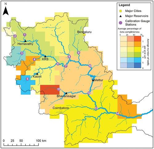
Table C1. Geological characteristics of geo-domains – for hydrogeology of the Cauvery catchment.

Domain	Domain – full	Topography/relief	Upper aquifer – regolith + fissured zones	Upper aquifer thickness	Lower aquifer – bedrock	Lower aquifer – permeability	Weathering thicknesses (m)	Fissured zone thickness (m)	Transmissivity (m^2/day)^a	Storage (%)^b	Specific yield	Yield (lps)	Source of evidence
GD1	Sedimentary rocks – delta	Low-lying (< 40 m asl) low relief – delta top	Not studied;pProbably dominated by sediment rather than weathered zone	Unknown; likely high	Sedimentary rocks of the Cauvery Delta	Likely to be highly permeable	Cretaceous: 50 Eocene: 80 Orathanadu: 30–70 Miocene main zone: 35 Pliocene: 10–35 Quaternary: 3–25		Min. range: 1–20 Max. range: 550–4500 (Cretaceous: <50 Eocene: 1600–1800 Orathanadu: 10–40 Miocene main zone: <1350 Pliocene: 50–40)		0.1–0.25	Min.: 9 Max.: 63	CGWB district reports Minor irrigation census well failure rates per district Krabbendam and Palamakumbura (2018)
GD2	Bangalore Plateau Dominated by peninsular Gneiss	High undulating plateau; gentle slopes, occasional low inselbergs; more dissected and steeper slopes along edges	Mainly saprock, saprolite only in low-lying areas;upper fissured zone (2–5 m) can be included in this Upper aquifer has sharp and regular boundary with lower bedrock aquifer	~ 5–10 m average; fairly uniform	Poorly fractured; upper layer of sheet joints (common and continuous) best modelled with upper aquifer Background jointing spacing > 5 m Fracture zones, withy spacing 1-5 km	Poor, likely poorly connected background fractures Large fracture zones may give locally high permeability	15–35		Min. range: 0.65–1 Max. range: 125–300	Saprolite: 1–6 Fissured zone: 1–3 Bedrock: 0.1	Saprolite: 0.05–0.1 Fissured zone: 0.01–0.03 Bedrock: 0.01	Min.: 0.1 Max.: 15	CGWB district reports Minor irrigation census well failure rates per district Benoit et al. (2017) working in Anantapur area just northeast of our study area Krabbendam and Palamakumbura (2018)
GD3	Charnockite domain Various granulite facies gneisses – without hydrous minerals	Strongly dissected, high-relief landscape (250–1400 m)	Mainly saprock and thin colluvium	Thin: <5 m	Poorly fractured; lack of sheeting joints Background jointing spacing > 1 m, but very tight Fracture zones, with spacing 1–5 km	Poor to very poor	19–35		Min. range: 0.65–20 Max. range: 250–300	0.015–2	Saprolite: 0.05–0.1 Bedrock: 0.005	Min.: 1 Max.: 2	CGWB district reports Minor irrigation census well failure rates per district Krabbendam and Palamakumbura (2018)
GD4	Deeply weathered domain Peninsular gneiss, granite, charnockite	High plateau (@ c. 900 m), very gentle “double-convex” relief; rivers have very low profiles	Thick and continuous saprolite layer > 5 m thick (clayey sand to sandy clay) Presumably underlain by an equally thick saprock layer	20–?30 m	Not studied; likely variable	Not studied; likely variable			Min. range: 0.65–1 Max. range: 1–125		Saprolite: 0.05 – 0.1 Fissured zone: 0.01–0.03 Bedrock: 0.01	Min.: 1 Max.: 15	CGWB district reports Minor irrigation census well failure rates per district Krabbendam and Palamakumbura (2018)
GD5	Granite domain Granite/granodiorite	Gently undulating with higher (100–400 m) inselbergs; often bare summits	Absent on bare tops; likely to be thicker (saprock and collucium in vales)	From 0 on bar tops to perhaps 15 m in vales	Poorly fractured; remarkable lack of sheeting joints. Background jointing spacing > 5 m Fracture zones, with spacing 1–5 km	Poor, likely poorly connected background fractures; large fracture zones may give locally high permeability	Oct-15	45	Min. range: 5–8.5 Max. range:300–550	Saprolite: 1–5 Fissured zone: 0.5–1.5 Bedrock: 0.3	Saprolite: 0.05–0.1 Fissured zone: 0.01–0.03 Bedrock: 0.01	Min.: 0.1 Max.: 9	CGWB district reports Minor irrigation census well failure rates per district Dewandel et al. (2010) Dewandel et al. (2006) Benoît et al. (2017) All the above are from work conducted in a granite domain in Kudaliar near Hyderabad, north of the study site Krabbendam and Palamakumbura (2018)
GD6	Lower catchment – hard-bedded Peninsular gneiss, granite, charnockite	Gently undulating, gradually descending (300 to 40 m) to delta; locally isolated inselbergs	Not studied; weathering front and thus regolith thickness highly variable Also alluvium widely present?	Not studied; likely highly variable	Variable, as contains peninsular gneiss, granite and charnockite	Not studied; variably poor?	20−35		Min. range: 0.65–8 Max. range: 125–550	0.015–1.5	Saprolite: 0.05–0.1 Fissured zone: 0.01–0.03 Bedrock: 0.01	Min.: 0.1 Max.: 27	CGWB district reports Minor irrigation census well failure rates per district Krabbendam and Palamakumbura (2018)
GD7	Mysore Plateau Peninsular gneiss and various supracrustal rocks	High undulating plateau (600–900 m) gentle slopes, no inselbergs Cauvery falls functions as high-level (c. 600 m) base level	Mainly saprock, saprolite only in low-lying areas; upper aquifer has gradual and irregular boundary with lower bedrock aquifer	~ 5–15 m average; highly variable	Variably fractured; locally densely fractured; mainly with vertical fractures	Fairly good in fractured areas; gradually decreasing with depth as fractures close	1–20		Min. range: 0.65 – 8 Max. range: 125–300 (Mysore district: Min. range: 8–20 Max. range: 500–1500)	Saprolite: 1–6 Fissured zone: 1–3 Bedrock: 0.1	Saprolite: 0.05–0.1 Fissured zone: 0.01–0.03 Bedrock: 0.01	Min.: 0.1 Max.: 18	CGWB district reports Minor irrigation census well failure rates per district Benoit et al. (2017) working in Anantapur area just northeast of our study area Krabbendam and Palamakumbura (2018)

^aRanges are based on the maximum (max.) and minimum (min.) values for each district within the geological domains based on data in CGWB district reports.

^bEffective porosity.

Figure D1. Daily hydrograph for gauged streamflow at sub-catchment 10, Biligundulu, which is upstream of the Mettur dam, and 12, Urachikottai, which is downstream of the Mettur dam (Fig. 1; Appendix B, Table B1) (India-WRIS 2020).

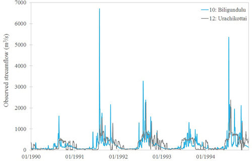
Figure D2. Daily hydrograph for sub-catchment 5, Munthankera (Fig. 1; Appendix B, Table B1), showing observed stream flow (India-WRIS 2020), and simulated streamflow from GWAVA and GWAVA-GW.

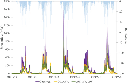
Figure D3. Daily hydrograph for sub-catchment 9, T. Bekuppe (Fig. 1; Appendix B, Table B1), showing observed stream flow (India-WRIS 2020), and simulated streamflow from GWAVA and GWAVA-GW.

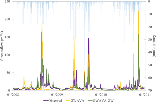
Figure D4. Daily hydrograph for sub-catchment 10, Biligundulu (Fig. 1; Appendix B, Table B1), showing observed stream flow (India-WRIS 2020), and simulated streamflow from GWAVA and GWAVA-GW.

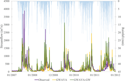
Figure D5. Observed (Central Ground Water Board 2009) and simulated (GWAVA-GW) groundwater abstractions over the sub-catchments (Fig. 1; Appendix B, Table B1).

Figure E1. Average depth to groundwater for the sensitivity runs, and average streamflow for the sensitivity runs, as a percentage of baseline results for each sub-catchment (1–11). The sensitivity variables are: anthropogenic demand, Sy (specific yield), and groundwater parameters λ and h_BF. The dot indicates the result when the sensitivity variable is increased.

India-WRIS [online], 2020. Available from: https://indiawris.gov.in/wris/#/ [ Accessed 1 September 2020].

 Google Scholar

Pai, D.S., et al., 2014. Developmentof a new high spatial resolution (0.25° X 0.25°) long period (1901-2010) daily gridded rainfall data set over India and its comparison with existing data sets over the region. Quarterly Journal of Meteorology, Hydrology & Geophysics, 65 (1), 1–18.

 Google Scholar

NASA JPL, 2013. NASA shuttle radar topography mission global 1arc second. Pasadena, CA, USA: LP DAAC.

 Google Scholar

Fischer, G., et al., 2008. Global agro-ecological zones assessment for agriculture. Rome, Italy: IIASA, Laxenburg, Austria and FAO.

 Google Scholar

Roy, P.S., et al., 2016. Decadal land use and land cover classifications across India, 1985, 1995, 2005. ORNL DAAC, Oak Ridge, Tennessee. doi:10.3334/ORNLDAAC/1336

 Google Scholar

India-WRIS, 2012. River basin atlas of India. Jodhpur: RSC-W, NRSC/ ISRO, Dept. of Space.

 Google Scholar

Robinson, T.P., et al., 2014. Mapping the global distribution of livestock. Plos One, 9 (5), e96084. doi:10.1371/journal.pone.0096084

 PubMed Web of Science ®Google Scholar

Census of India, 2001. Provisional population totals. Government of India.

 Google Scholar

Government of Karnataka, 2014. Watershed development department” annual report 2013-2014. Government of Karnataka.

 Google Scholar

Krabbendam, M. and Palamakumbura, R., 2018. Gneiss, fractures and saprolite: field geology for hydrogeology of the central Cauvery Catchment, south India. Nottingham, UK: British Geological Survey: NERC Open Research Archive.

 Google Scholar

Benoit, D., et al., 2017. Geophysical signature location in the South-West of Chad: structural implications. Journal of Geology & Geophysics, 7 (1). doi:10.4172/2381-8719.1000319

 Google Scholar

Dewandel, B., et al., 2010. Development of a tool for managing groundwater resources in semi-arid hard rock regions: application to a rural watershed in South India. Hydrological Processes, 24 (19), 2784–2797. doi:10.1002/hyp.7696

 Web of Science ®Google Scholar

Dewandel, B., et al., 2006. A generalized 3-D geological and hydrogeological conceptual model of granite aquifers controlled by single or multiphase weathering. Journal of Hydrology, 330 (1–2), 260–284. doi:10.1016/j.jhydrol.2006.03.026

 Web of Science ®Google Scholar

Central Ground Water Board, 2009. District ground water brochures [online]. Available from: http://cgwb.gov.in/District-GW-Brochures.html [ Accessed 1 February 2021].

 Google Scholar