Validation of hybrid angular spectrum acoustic and thermal modelling in phantoms

Figures & data

Table 1. Parameters for acoustic and thermal simulations and their uncertainties for Monte Carlo analysis.

Simulation parameter	Symbol	Phantom type (% milk)	Mean (μ)	Measurement uncertainty (σXj)	Uncertainty determination
Acoustic power (W)	P		6.3	1.05%	Error propagation of force balance-measured efficiency and reported experimental transducer electrical output
			7.9
Acoustic attenuation (Np/cm @ 1 MHz)	α	10%	0.015	16%	Difference between through-transmission and radiation force balance measurements (n = 3)
		30%	0.027
		50%	0.042
		70%	0.053
Speed of sound (m/s)	c	10%	1540.0	0.10%	Standard deviation of experimental measurement
		30%	1552.0
		50%	1560.3
		70%	1571.7
Density (kg/m^3)	ρ	10%	1022	0.8%	Standard deviation of experimental measurement
		30%	1050
		50%	1040
		70%	1050
Volumetric heat capacity (kJ/m^3·°C)	VHC	10%	3404	10%	Manufacturer reported error of measurement device
		30%	3361
		50%	3371
		70%	3381
Thermal conductivity (W/m·°C)	κ	10%	0.554	10%	Manufacturer reported error of measurement device
		30%	0.545
		50%	0.565
		70%	0.525

Figure 1. Experimental set-up for FUS sonications in homogeneous gelatin phantoms with real-time volumetric MRTI as shown in an axial T1-weighted MR image. (A) 256-element phased-array transducer is positioned below the phantom cylinder, coupled with room-temperature degassed, deionised water. The geometric focus was placed 19.5 mm into the base of the phantom. The MRTI image slab was oriented perpendicular to the direction of FUS beam propagation, with slices centred at the geometric focus. The base of the MRTI volume was 7.5 mm above the bottom of the phantom.

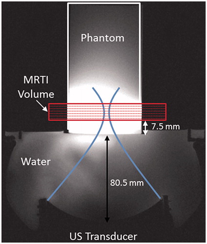
Table 2. Fixed acoustic and thermal simulation parameters and simulation computation time.

Acoustic (HAS)		Thermal (PBHE)
Transducer frequency	940 kHz	Time step	0.08 s
Focus depth	19.5 mm	Heating time	18.16 s
		Perfusion term	0 kg/(m³·s)
		Boundary condition	Constant temperature
Model size	647 × 343 × 280	Model size	647 × 343 × 280
Model resolution (isotropic)	0.25 mm	Model resolution (isotropic)	0.25 mm
Average computation time	32.1 s	Average computation time	35.3 s

Figure 2. Average peak temperature rise achieved in the simulated (dashed, n = 1) and experimental (solid, n = 3) temperature profiles, with experimental error bars representing one standard deviation. Results are plotted as a function of milk concentration of the gelatin phantoms for both FUS sonication powers: 6.3 W (blue, circles) and 7.9 W (red, triangles).

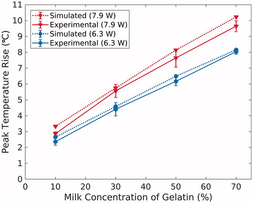
Table 3. Comparison of experimental (n = 3) and simulated (n = 1) temperature profiles at temporal peak of HIFU heating.

	Spatial peak temperature rise (°C)		Transverse profile FWHM (mm)		Longitudinal profile FWHM (mm)		MRTI Data (°C)
Milk composition	Experimental	Simulation	Experimental	Simulation	Experimental	Simulation	Average noise^a	Average SNR^b
6.3 W
10%	2.36 ± 0.21	2.66	2.73 ± 0.08	2.76	16.74 ± 0.81	19.00	0.240	9.84
30%	4.41 ± 0.42	4.58	2.88 ± 0.09	2.76	18.14 ± 0.33	19.00	0.156	24.69
50%	6.17 ± 0.26	6.49	2.77 ± 0.1	2.78	16.92 ± 0.46	19.08	0.160	32.39
70%	8.04 ± 0.16	8.15	2.78 ± 0.05	2.74	17.23 ± 0.50	18.92	0.201	40.13
7.9 W
10%	2.87 ± 0.12	3.33	2.77 ± 0.19	2.76	17.52 ± 0.12	19.00	0.177	13.01
30%	5.57 ± 0.41	5.75	2.83 ± 0.12	2.76	16.84 ± 0.79	19.00	0.186	27.31
50%	7.64 ± 0.57	8.14	2.79 ± 0.12	2.78	17.88 ± 0.94	19.08	0.172	36.15
70%	9.64 ± 0.34	10.23	2.82 ± 0.06	2.74	17.39 ± 0.43	18.92	0.151	54.32
Average % error (Ei)	+6.9 ± 5.0%		–1.9 ± 1.5%		+7.45 ± 3.0%		--

^a The standard deviation in time of a 36-voxel non-heated region in the phantom (n = 3).

^b Experimental Peak Temperature Rise/Standard Deviation (n = 3).

Figure 3. Transverse (top) and longitudinal (bottom) profiles of mean experimental (circle, black) and simulated (square, blue) temperature data in 50% milk composition phantoms at 7.9 W. Depicted transverse profiles are along the short-axis of the transducer face. For longitudinal profiles, the transducer is located to the left of the profiles. Experimental and simulated profiles are compared at multiple times points during heating (t = 3.04 and t = 9.76 s), at the time of experimental peak temperature rise (t = 16.48 s), and during cooling (t = 23.20 s and t = 29.92 s). Simulated profile resolution is down-sampled to 0.5 mm isotropic to match experimental spatial resolution.

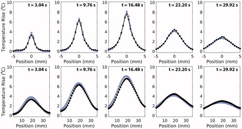
Figure 4. Average percent error in spatio-temporal peak temperature rise (black), transverse (blue, dashed) FWHM, and longitudinal (red, dotted) FWHM for all phantoms and sonication powers is plotted throughout FUS heating and cooling (n = 8; error bars= ± one standard deviation). The shaded regions represent time-points during which the average spatial SNR in the MRTI experimental data across all phantoms was ≤ 20.

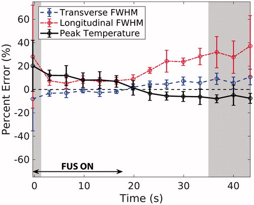
Figure 5. Temporal temperature curves of the peak temperature voxel from experimental (black, solid) and corresponding simulated (blue, dotted) temperatures for (a) 10%, (b) 30%, (c) 50%, and (d) 70% milk at 7.9 W sonication. Experimental error bars represent one standard deviation (n = 3). The shaded envelope represents one standard deviation of the MC analysis. The black dotted lines represent the high and low extremes of the MC analysis.

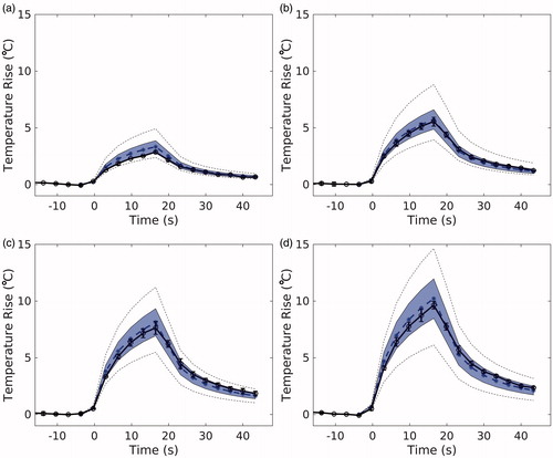
Table 4. Linear regression analysis of all MC Simulations (n = 568).

		Peak temp rise		Transverse FWHM		Longitudinal FWHM
		R^2	SRC^a	R^2	SRC	R^2	SRC
		0.979		0.991		0.991
Acoustic attenuation	α		0.825		0.024		0.078
Speed of sound	c		0.053		–0.002		–0.078
Acoustic power	P		0.275		0.001		0.001
Density	ρ		0.040		–0.004		0.018
Thermal conductivity	κ		–0.158		0.787		0.787
Volumetric heat capacity	VHC		–0.074		–0.734		–0.728

^a SRC: Standardized Regression Coefficient.

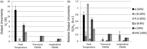
Figure 6. Output uncertainty (U_j) and relative output uncertainty ($U_{\mathrm{j}}{\sigma }_{{\mathrm{X}}_{\mathrm{j}}}$) for three different output metrics of the MC simulations. (a) U_j when each parameter is varied individually (as specified in the legend). (b) $U_{\mathrm{j}}{\sigma }_{{\mathrm{X}}_{\mathrm{j}}}$ comparing the relative impact of each parameter on U_j. Output uncertainties were averaged over all phantoms and power levels. Error bars represent one standard deviation.