Exploring the potential of the dynamic hysteresis loops via high field, high frequency and temperature adjustable AC magnetometer for magnetic hyperthermia characterization

Figures & data

Figure 1. (a) Solenoid coil (b) Sliced plane of the solenoid coil. Spatial distribution of the current density in the cross section of three turn solenoid with: (c) 5 mm turn pitch and (d) 10 mm turn pitch calculated by Finite Element Method (FEM) when 1 A intensity and 10 kHz frequency circulates across the coil.

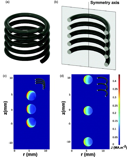
Figure 2. (a) Energy efficiency as a function of different number of turns calculated by FEM for 1, 2 and 3 winding layers coil. The simulations were performed supplying the coil with a 1 kW power amplifier and an AC current of 1 MHz frequency. (b) Equivalent resistance of the coil as function of number of turns for 1, 2, and 3 winding layers.

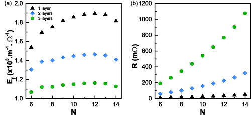
Figure 3. (a) Main coil cross section image showing the air flow system (b) Scheme of the air temperature controller.

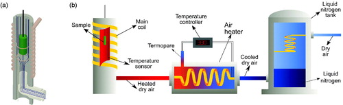
Figure 4. Complete scheme of the AC magnetometer set up.

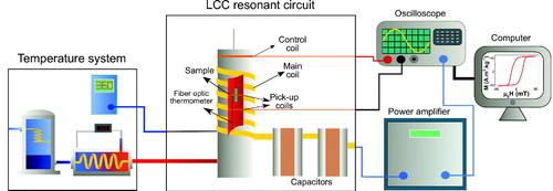
Figure 5. TEM images of samples (a) A, (b) B, (c) C and (d) D together with their corresponding size distributions. Scale bar 50 nm.

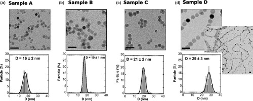
Figure 6. First row: DC hysteresis loops at 5 K (red line) and 300 K (black line) for samples (A) A, (b) B, (c) C and (d) D. Second row: ZFC-FC curves (black line) together with derivatives of ZFC magnetization (blue line) for samples (e) A, (f) B, (g) C and (h) D.

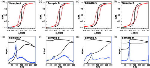
Figure 7. AC hysteresis loop of sample (a) A, (b) B, (c) C and (d) D taking at room temperature (RT) under magnetic field of 90 mT at 134 kHz. Note that all the samples saturate almost at 50 mT. As size of the sample increase, the loops broaden obtaining a square shape loop in the sample D.

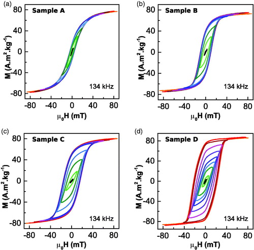
Figure 8. SAR versus field intensity curves obtained from the area of AC hysteresis loops under the field frequency of 134 kHz at liquid state. Measurements are performed at room temperature in liquid state for four samples.

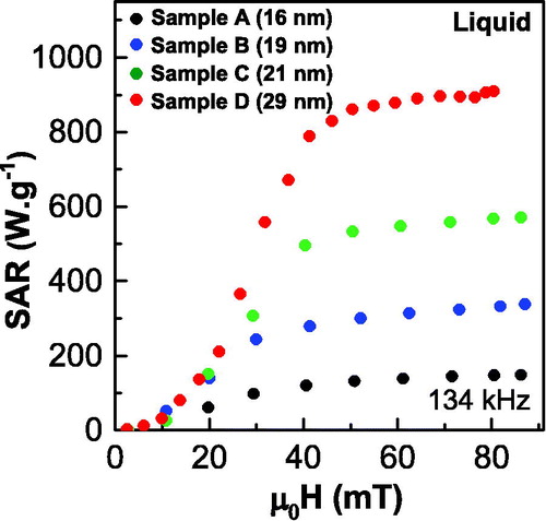
Figure 9. AC hysteresis loops of sample (a) A, (b) B, (c) C and (d) D under magnetic field of 90 mT and frequency of 134 kHz in room temperature/liquid state (black) and frozen state (red).

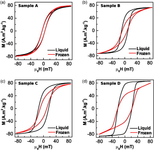
Figure 10. SAR versus field intensity curves obtained from the area of AC hysteresis loops under the field frequency of 134 kHz at frozen state. The dots indicate the experimental results and the lines their corresponding simulations using Stoner–Wohlfarth model based theories (SWMBTs).

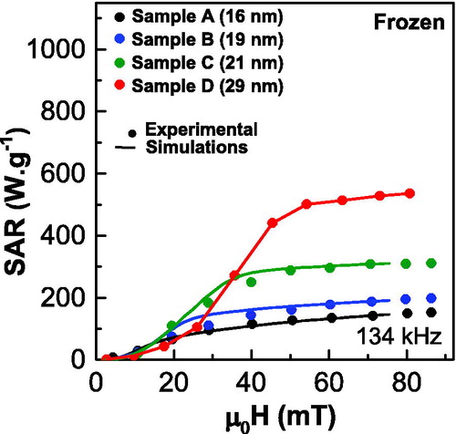
Figure 11. First row: AC hysteresis loop of sample (a) A, (b) B, (c) C and (d) D at 134 kHz (red), 561 kHz (green), 835 kHz (blue) and DC (black) in frozen media at 30 mT. Second row: SAR/f versus field intensity curve obtained from the area of AC hysteresis loops at 134 kHz (red), 561 kHz (green) and 835 kHz (blue) of sample (e) A, (f) B, (g) C and (h) D. The dots indicate measurements performed in frozen solutions and lines their corresponding simulations by using SWMBTs [49].

Figure 12. SAR/f versus particles’ size curves at (a) 22 mT (b) 28 mT and (c) 45 mT magnetic field intensities and 134 kHz (black line), 561 kHz (blue line) and 835 kHz (green line) frequencies.

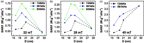
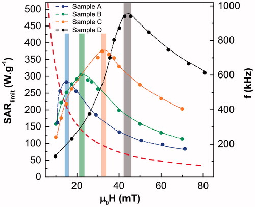
Figure 13. Maximum achievable SAR, SAR_limit, under the Hergt criterion for all the samples. The red dashed curve is the acceptable maximum frequency, f_limit(H) = 5 × 10⁹Am⁻¹s⁻¹/H, for a given magnetic field intensity following the Hergt criterion. The optimal excitation intensity to get the maximum SAR_limit value is indicated with colored bars (each color corresponds to one of the samples). The intersection of the red dashed curve and the colored bar of each sample shows the optimal frequency for obtaining the maximum SAR_limit value.

Carrey J, Mehdaoui B, Respaud M. Simple models for dynamic hysteresis loop calculations of magnetic single-domain nanoparticles: application to magnetic hyperthermia optimization. J Appl Phys. 2011;109(8):083921.

 Web of Science ®Google Scholar