
Figures & data
Table 1. concentrations of glycerol, EC, and oil for the two optimized recipes.
Figure 1. Schematic of the measurement setup for the dielectric properties (DAK-TL2).
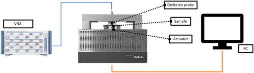
Figure 2. Graphical representation of the geometry adopted for the simulation of an EM radiative system (left) and of a capacitive system (right).
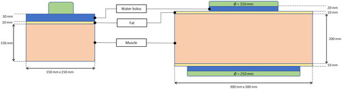
Table 2. Dielectric properties used in the simulation studies for both radiative and capacitive systems.
Figure 3. Top left: schematic representation of the experimental setup. The probes position and the geometrical dimensions are indicated. Bottom left: position of the temperature sensors for the probes M1-3, located at 1 cm below the muscle surface, with respect to the antenna aperture (red dotted line). On the right: picture of the same setup.
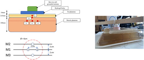
Figure 4. A phantom sample used for the QA experimental verification. The material can be easily handled without damaging its structure.
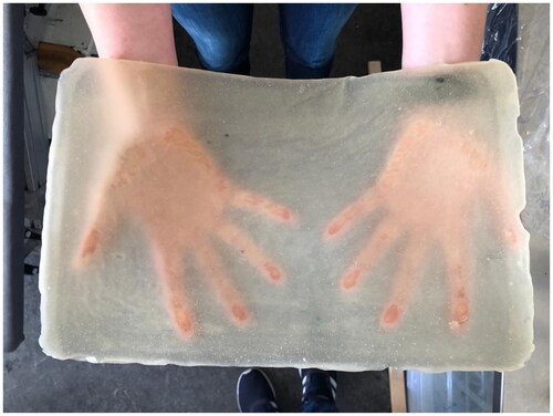
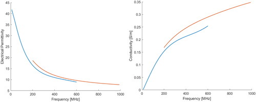
Figure 5. Average permittivity (left) and electrical conductivity (right) of the phantom, using a DAK12-TL2 (green solid line) and a DAK3.5-TL2 (blue solid line), with their confidence intervals. The dashed lines represent the dielectric properties of the average infiltrated fat tissue (red), and non-infiltrated fat tissue (yellow), both taken from the IT’IS database. The corresponding shaded areas indicate the uncertainty of dielectric probe measurements. Two vertical markers are positioned at 434 MHz and at 915 MHz.
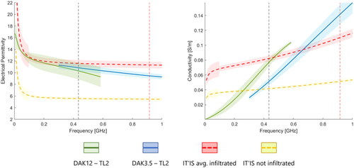
Table 3. Average permittivity and conductivity measured values for two different phantom formulations (glycerol concentration: 57 wt% and 52 wt%). The data are reported for two common operating frequencies in HT, 434 MHz and 915 MHz.
Table 4. Measured thermal properties of the phantom at room temperature.
Figure 6. G' (solid line) and G'' (dashed line) as a function of temperature for different glycerol content phantoms: 0 wt% (left) and 65 wt% (right). The samples were first cooled from 130 °C to 20 °C (blue) and then heated to reach again 130 °C (green).
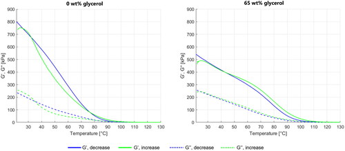
Table 5. G′ and tan δ at T = 20 and 39 °C for EC and EC glycerol gels. The moduli values were recorded at f = 1 Hz and strain = 0.5%. The different values given are the value obtained upon cooling (C) and heating (H).
Table 6. Gel-setting temperature calculated for the different phantom samples with increasing glycerol content.
Table 7. EFS, TEFS and TEPD values calculated from the simulated SAR and temperature distribution for a capacitive and a radiative system, adopting different dielectric properties for the fat layer (values from the database, plus lower, higher, and average values measured in the phantom). The percentage difference with respect to the values computed using the IT’IS based fat phantom model is also shown.
Figure 7. Contour plots of the temperature increase within a fat-muscle phantom after 6 min of heating with a single antenna radiative system (top row) and a two electrodes capacitive system (bottom row), as described in section 2.5.1. Left column: XY plan view at 1 cm depth in the muscle phantom, where the red dotted lines indicate the boundaries of the TEFS and the contours of the antenna and the top electrode are represented as white dotted lines. Right column: XZ view. Here, the boundaries between fat/muscle/bolus are shown as black dotted lines.
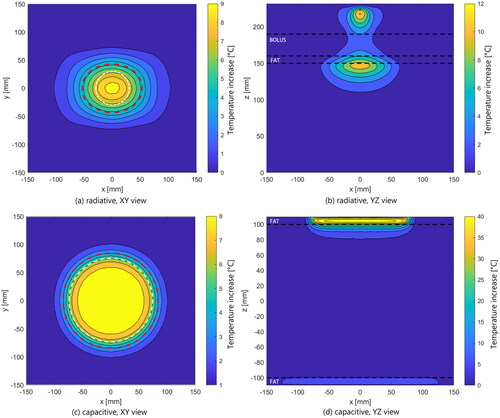
Figure 8. Temperature increase recorded over 6 min by fiber-optic temperature probes at different measurement points. On the right side, the location of the sensors (top) and the location of the probes within the layered phantom (bottom).
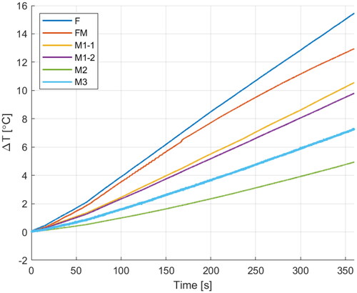
Figure 9. IR camera thermal images capturing the temperature distribution (top row) and simulated temperature levels after 6 min of exposure at 87 W (bottom row) at different interfaces. From the left to right: Fat/Fat, Fat/Muscle, Muscle/Muscle (1 cm deep). The markers on the thermal images correspond to the approximate position of the temperature sensors during the experiment.
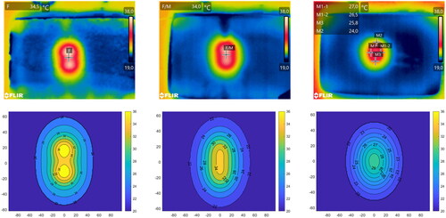
Figure 10. Comparison between the measured (orange line) and simulated (blue line) temperature increase along the y = 0 axis (left panel) and the x = 0 axis (right panel).
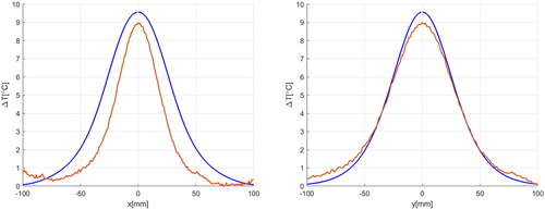
Figure A1. Permittivity and conductivity measured on a sample of pure glycerol using the DAK12 – TL2 (blue line) and the DAK3.5 – TL2 (orange line) probes.
Data availability statement
Raw data were generated at Chalmers University of Technology, Göteborg, and Eramsus MC, Rotterdam. Derived data supporting the findings of this study are available from the corresponding author H.D.T. on request.