Case study: shipping trend estimation and prediction via multiscale variance stabilisation

Figures & data

Figure 1. Monthly Cyprus shipping credit flows.

Figure 2. Estimated mean–variance relationship for Cyprus shipping credit flows. Black dots show (absolute value of) finest scale mother wavelet coefficients against their corresponding fathers illustrating Equation  (4(3) $d_{1,1}=(X_1-X_2)/2d_{1,2}=(X_3-X_4)/2.$(3) ). Estimate of h is shown by solid line. For visual guidance only the grey dot-dash line shows $\mathrm{sd}=\mathrm{mean}$ and the grey dashed line is the straight line closest to $\hat{h}$ approximately equal to $\mathrm{sd}=\mathrm{mean}-0.287$.

Figure 3. Monthly variance-stabilised Cyprus shipping credit flows, $y_t$ by transformation: (a) Box–Cox ; (b) log ; (c) square root; (d) data-driven Haar–Fisz, vertically shifted down by the constant 45141433.

Figure 4. Smoothed Cyprus shipping credit flows. Black dots show actual flows (as in Figure 1). Red line is data-driven Haar–Fisz stabilised estimate with 50% (dark blue) and 95% (light blue) approximate confidence intervals. Green line is standard smoothing spline estimate of credit flows.

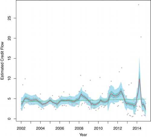
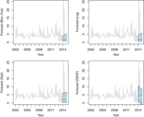
Figure 5. Forecasts of Cyprus shipping credit flows for h=12 steps ahead obtained via four different transform methods. Grey line shows actual flow (as in Figure 1). Solid blue line shows the forecasts from one to h=12 steps ahead and the blue polygon shows the (nominal) 95% prediction interval.

Table 1. Mean squared prediction error for the four transformations for varying forecasting horizons.

h	3	6	9	12	15	18	21	24
Box–Cox	0.86	1.21	1.98	2.73	2.19	1.76	1.50	1.35
Log	0.97	1.32	1.97	2.71	2.15	1.70	1.50	1.35
Sqrt	2.15	1.60	2.00	2.65	2.01	1.70	1.50	1.34
DDHF	1.96	1.23	3.44	2.46	2.05	1.70	1.48	1.37

Table 2. Empirical percentage coverage of 95% prediction intervals based on transformed ets forecasting based on eight different forecasting horizons, h.

h	3	6	9	12	15	18	21	24
Box–Cox	33	50	56	83	81	61	38	30
Log	66	50	56	83	81	50	48	33
Sqrt	33	50	56	83	53	50	43	46
DDHF	33	83	89	83	67	67	71	42