Bodily feelings and aesthetic experience of art

Figures & data

Figure 1. Overview of the study design for Experiments 1–3. Sample paintings from top to bottom: Kaski (Eero Järnfelt), Morsiamen laulu (Gunnar Berndtson), Leikkiviä poikia rannalla (Albert Edelfelt), Toipilas (Helene Schjerfbeck).

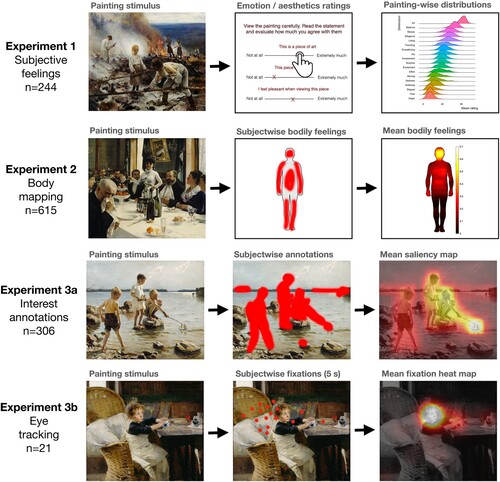
Table 1. Summary of the number of stimuli and subjects used in each experiment. Note that stimuli in Experiment 1 and 2 were the same, and a subset of those was used in Experiments 3a–b.

	n (stimuli)	n (subjects)	n (stimuli per subject)
Experiment 1: Subjective feelings	336	244	22 (mean)
Experiment 2: Bodily sensations	336	615	24
Experiment 3a: Interest annotations	60	306	30
Experiment 3b: Eye tracking	60	21	60

Figure 2. Frequency distributions of the rated dimensions of the art pieces.

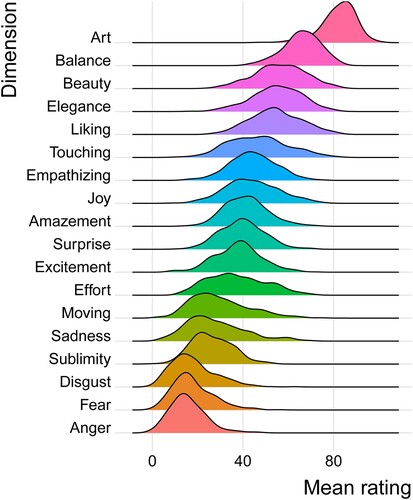
Figure 3. Pearson correlations between the rated dimensions. Black outlines show the clustering of the rated dimensions.

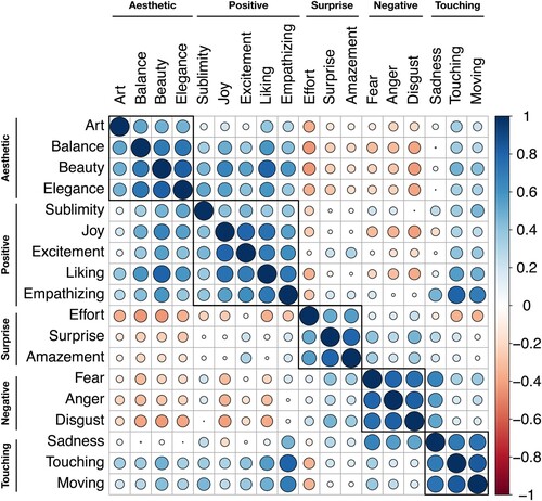
Figure 4. Regression coefficients and their 95% confidence intervals for models predicting liking (A) and art-like qualities (B) of the artworks in the stepwise regression models. Coefficients are arranged in ascending order separately for each model.

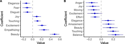
Figure 5. Bodily maps of aesthetic and emotional experiences while viewing art. The maps show the statistically significantly activated regions across subjects for each feeling. The maps are arranged as a function of the mean proportion of significant pixels, and thresholded at p < 0.005, FDR corrected. Colourbar indictaes the t statistic range.

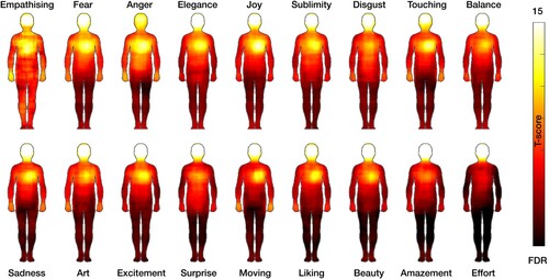
Figure 6. Bodily and mental components and aesthetic and emotional evaluations of art. Mean Pearson correlation between bodily (A) and mental (B) sensations and the aesthetic and emotional qualities of the paintings. Red lines show the area of nonsignificant correlations.

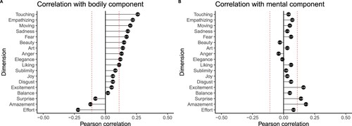
Figure 7. Manually annotated mean saliency maps (A) and fixation heatmaps (B) for 4 representative paintings. Colourbars show the proportion of subjects colouring each area (top) and the fixation density estimate (B). Sample paintings from left to right: Kaiku (Ellen Thesleff), Dans le Lit, le Baiser (Henri de Toulouse-Lautrec), Maisema Kolilta (Eero Järnfelt), Composition 8 (Vassily Kadinsky).

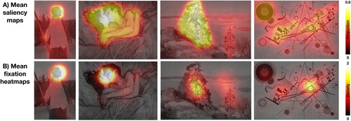
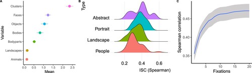
Figure 8. Summary of the annotation results. Means ± standard errors of mean for the number of clusters and the frequency of the contents for the clusters (A). Distribution of intersubject similarity of the painting annotations (n = 336) for different painting types (B). Mean ± standard error of mean intsersubject correlation (Spearman) between the interest annotations and gaze-based saliency maps from 1–20 first fixations (C).

Data availability statement

Data are available from the corresponding author per request.