Testing continuity in a Michigan (USA) river using the organic biomass of adult Ephemeroptera, Plecoptera, and Trichoptera

Figures & data

Figure 1. Location of the 13 sampling sites along the continuum of the Pine River. Sampling site numbers correspond to Table 1 and Table 2. White line approximates the border of the Pine River watershed. Base map © Google, TerraMetrics.

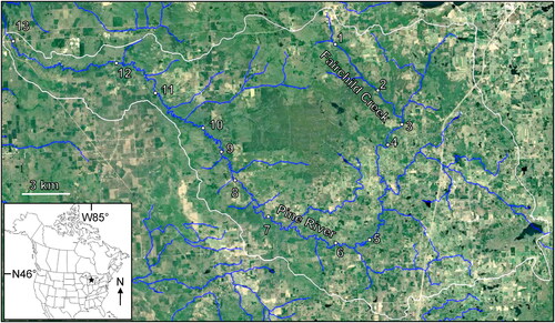
Table 1. Each site’s position from upstream (1) to downstream (13), GPS coordinates, and the number of samples collected at that site. Site numbers are in Figure 1.

Site number	Site name	GPS coordinates	Number of samples
1	Fairchild Creek	44°12′30”N, 85°34′22”W	4
2	Fr 5498	44°10′21”N, 85°31′55”W	4
3	Southern Fairchild	44°08′48”N, 85°30′32”W	4
4	22 Mile Rd	44°07′57”N, 85°31′28”W	3
5	17 Mile Rd	44°03′48”N, 85°32′53”W	4
6	Raymond Rd	44°03′44”N, 85°34′59”W	3
7	Skookum	44°05′03”N, 85°39′04”W	4
8	Walker Bridge	44°06′44”N, 85°40′60”W	4
9	Lincoln Bridge	44°08′00”N, 85°41′44”W	3
10	Elm Flats	44°90′05”N, 85°42′48”W	4
11	Dobson Bridge	44°10′45”N, 85°45′38”W	3
12	Peterson Access	44°12′11”N, 85°47′57”W	3
13	Manistee	44°13′23”N, 85°54′15”W	4

Table 2. Mean specimen abundance values for each of the 50 EPT taxa caught in this study, rounded to the nearest whole number. Site numbers correspond to Table 1 and Figure 1.

Site number
Taxon	1	2	3	4	5	6	7	8	9	10	11	12	13
EPHEMEROPTERA
Baetidae
Acentrella	0	0	0	0	0	0	0	0	<1	0	0	0	0
Baetis	3	2	3	4	6	12	5	5	14	4	15	21	12
Caenidae
Caenis	1	2	10	10	20	19	21	8	33	42	37	61	183
Ephemerellidae
Ephemerella	2	0	1	4	2	3	8	10	13	25	12	19	1
Ephemeridae
Hexagenia	0	0	0	<1	1	3	1	3	2	4	8	10	33
Heptageniidae
Stenonema	<1	1	1	2	2	3	4	4	4	5	4	<1	0
Stenacron	0	0	0	0	0	0	0	<1	0	<1	0	0	0
Isonichiidae
Isonychia	1	0	1	1	2	0	1	3	6	1	10	17	25
Leptophlebiidae
Paraleptophlebia	0	1	1	0	2	0	4	1	0	0	0	0	0
PLECOPTERA
Chloroperlidae
Alloperla	<1	1	0	1	<1	1	0	<1	1	1	0	0	0
Nemouridae
Amphinemoura	1	1	1	2	1	<1	1	2	1	1	1	<1	0
Perlidae
Paragnetina	0	0	0	0	0	<1	0	1	0	0	0	0	0
Perlodidae
Isoperla	1	3	3	5	11	9	18	19	6	25	7	35	10
Pteronarcyiidae
Pteronarcys	0	<1	<1	<1	0	0	0	0	0	0	0	0	0
TRICHOPTERA
Brachycentridae
Brachycentrus	2	3	1	0	16	14	44	70	78	102	47	46	8
Micrasema	0	0	1	1	30	62	18	63	96	157	56	18	11
Dipseudopsidae
Phylocentropus	0	0	0	0	0	0	0	0	0	0	0	<1	0
Glossosomatidae
Agapetus	<1	0	0	0	0	0	0	0	<1	0	0	0	0
Glossosoma	3	0	10	5	9	46	42	43	47	5	4	14	0
Helicopsychidae
Helicopsyche	0	<1	<1	10	24	1	3	0	0	0	0	0	0
Hydropsychidae
Cheumatopsyche	24	1	29	18	4	23	14	11	2	2	1	5	54
Hydropsyche	9	58	104	118	109	140	194	150	331	181	367	115	398
Potamyia	0	0	0	0	0	0	0	0	0	0	<1	1	0
Hydroptilidae
Agraylea	0	0	0	0	2	1	2	<1	<1	1	<1	0	5
Other hydroptilids	3	156	39	43	106	213	254	293	304	224	286	143	260
Lepidostomatide
Lepidostoma	3	136	161	617	1142	846	1125	473	970	950	606	48	22
Leptoceridae
Ceraclea	2	4	2	2	759	484	629	642	699	464	471	246	828
Leptocerus	<1	2	1	8	19	3	1	1	0	0	3	511	2231
Mystacides	0	0	0	<1	2	1	2	1	0	1	0	0	<1
Nectopsyche	0	0	0	0	0	1	<1	2	2	4	0	1	48
Oecetis	1	2	1	9	15	14	21	28	37	33	21	2	47
Setodes	0	0	0	0	0	0	0	<1	1	0	0	<1	0
Triaenodes	1	<1	1	3	20	19	11	1	4	2	14	7	12
Limnephilidae
Anabolia	0	0	0	0	0	<1	3	1	0	0	<1	0	<1
Limnephilus	<1	1	0	0	0	<1	<1	1	1	1	<1	0	0
Platycentropus	3	0	0	0	1	<1	0	0	0	0	0	<1	0
Pycnopsyche	5	8	1	5	2	2	1	5	2	11	4	1	1
Molannidae
Molanna	0	<1	<1	1	<1	<1	1	<1	0	1	<1	0	0
Philopotamidae
Chimarra	1	<1	<1	1	2	1	2	3	4	1	1	2	26
Dolophilodes	9	6	4	23	1	1	<1	2	0	1	0	0	0
Phryganeidae
Banksiola	0	2	2	2	2	2	4	1	2	1	1	0	1
Phryganea	0	<1	0	0	1	1	<1	1	<1	0	<1	0	2
Ptilostomis	1	<1	<1	<1	0	1	<1	1	1	<1	0	0	1
Polycentropodidae
Cernotina	0	0	0	0	1	0	0	0	0	0	0	0	0
Cyrnellus	0	0	0	0	0	0	0	0	0	0	0	0	4
Neureclipsis	0	0	1	8	1	0	1	2	2	3	1	0	2
Nyctiophylax	0	0	2	37	2	2	20	6	6	21	14	10	37
Plectrocnemia	0	0	2	11	1	2	2	0	0	2	1	0	12
Polycentropus	2	3	10	16	2	3	5	7	3	9	4	5	3
Psychomyiidae
Lype	7	17	16	6	11	5	10	4	4	4	20	1	2
Psychomyia	1	2	19	4	7	52	27	20	15	30	17	4	212

Figure 2. NMDS ordination of the 13 sampling sites based on mean EPT FFG biomass per site. P-values from a Monte Carlo test of non-random ordination structure. Arrow lengths denote strength of correspondence of FFG biomass with axis 1 values, only r² > 0.50 shown. N = 3–4 per site (Table 1).

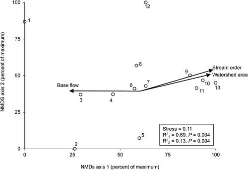
Figure 3. Second degree polynomial regression models of mean (±SE) AFDM (dependent variable) based on axis 1 scores from Figure 2 (independent variable) for filtering collectors (A), gathering collectors (B), predators (C), scrapers (D), shredders (E). Summary equations and R² values in separate box. Each marker represents the mean (±SE) of 1 of the 13 sampled sites. N = 3–4 per site.

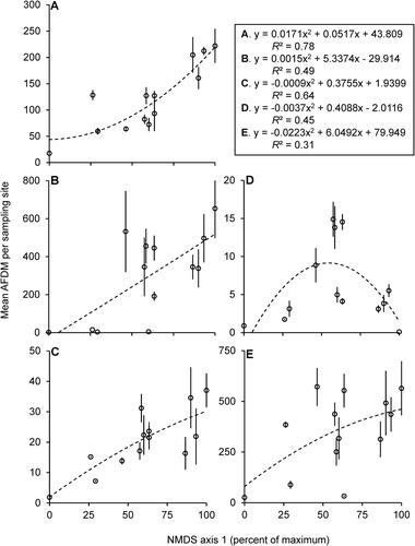
Figure 4. Second degree polynomial regression model of mean (±SE) number of EPT genera caught (dependent variable) based on axis 1 scores from Figure 2 (independent variable) for the 13 sampling sites, with summary equation and R² values. Each marker represents the mean (±SE) of 1 of the 13 sampled sites. N = 3–4 per site.

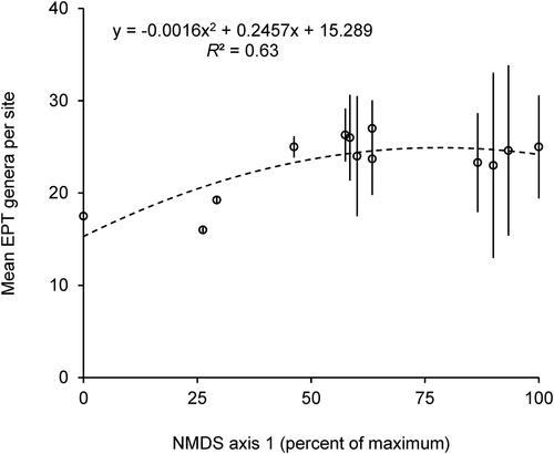
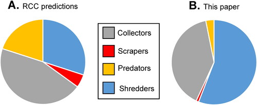
Figure 5. Approximate relative biomass of each FFG as predicted by Vannote et al. (1980) for 1st–4th order streams (A), compared to the data in our study when expressed as relative determined biomass (B).

Vannote RL, Minshall GW, Cummins KW, Sedell JR, Cushing CE. 1980. The river continuum concept. Can J Fish Aquat Sci. 37(1):130–137.

 Web of Science ®Google Scholar

Data availability statement

Data are available on the Open Science Framework site: https://osf.io/nqfdh/.