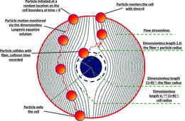
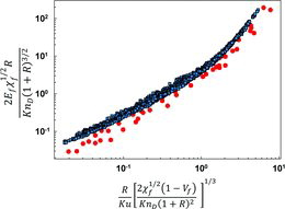
2,719
Views
14
CrossRef citations to date
0
Altmetric
Original Articles

The Single-Fiber Collision Rate and Filtration Efficiency for Nanoparticles I: The First-Passage Time Calculation Approach

, &
Pages 875-885 | Received 24 Sep 2013, Accepted 10 Jun 2014, Published online: 11 Aug 2014

Figures & data

FIG. 1. Schematic describing the MFPT approach to determine dimensionless collision kernels. Relevant dimensionless length scales for calculation are labeled, and a depiction of particle motion is provided.
FIG. 2. The dimensionless collision kernel as function of the diffusive Knudsen number for a cylindrical cell model in the absence of fluid flow (χf = 0), as determined by MFPT calculations. Circles (red): Vf = 6.83 × 10⁻⁴; squares (blue): Vf = 3.42 × 10−3; long dashed line (red): EquationEquation (5b) calculated values with Vf = 6.83 × 10⁻⁴; short dashed line (blue): EquationEquation (5b) calculated values with Vf = 3.42x 10⁻³; solid line (black): Equation (6b) calculated values.
FIG. 2. The dimensionless collision kernel as function of the diffusive Knudsen number for a cylindrical cell model in the absence of fluid flow (χf = 0), as determined by MFPT calculations. Circles (red): Vf = 6.83 × 10⁻⁴; squares (blue): Vf = 3.42 × 10−3; long dashed line (red): EquationEquation (5b)[5b] calculated values with Vf = 6.83 × 10⁻⁴; short dashed line (blue): EquationEquation (5b)[5b] calculated values with Vf = 3.42x 10⁻³; solid line (black): Equation (6b) calculated values.
FIG. 3. Values of the parameter (H/HC – 1) with H determined from MFPT calculations and HC calculated with EquationEquation (5b) for (a) Vf = 0.01 and (b) Vf = 0.07. Circles (red): R = 0; squares (blue): R = 0.03; triangles (yellow): R = 0.10. Plots such as those displayed are used to determine the coefficients C1 and C2 as functions of Vf and R.
FIG. 3. Values of the parameter (H/HC – 1) with H determined from MFPT calculations and HC calculated with EquationEquation (5b)[5b] for (a) Vf = 0.01 and (b) Vf = 0.07. Circles (red): R = 0; squares (blue): R = 0.03; triangles (yellow): R = 0.10. Plots such as those displayed are used to determine the coefficients C1 and C2 as functions of Vf and R.

TABLE 1. Values of the coefficients (a) C1 and (b) C2 determined from regressions, as functions of R and Vf
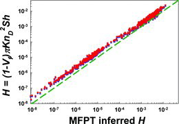
FIG. 4. A comparison of the dimensionless collision kernels inferred from MFPT calculations to those calculated from EquationEquation (12a) (Modeled H). Circles (red): C1 and C2 determined Equations (13a) and (13b). Squares (blue): tabulated C1 and C2 values used for calculations. The central dashed line (black) denotes 1:1 values, whereas the outer dashed lines (gray) denote 1:1.25 and 1:0.75 values.
FIG. 4. A comparison of the dimensionless collision kernels inferred from MFPT calculations to those calculated from EquationEquation (12a)[11b] (Modeled H). Circles (red): C1 and C2 determined Equations (13a) and (13b). Squares (blue): tabulated C1 and C2 values used for calculations. The central dashed line (black) denotes 1:1 values, whereas the outer dashed lines (gray) denote 1:1.25 and 1:0.75 values.
FIG. 5. Depth filtration predicted single-fiber efficiencies as compared to those inferred from MFPT calculations. (a) Calculated with R ≤ 0.03; (b) calculations with R ≥ 0.07. Circles (red): diffusion collection only (Equation (14a)); squares (blue): combined diffusion and interception collection (Equation (14a) + EquationEquation (14c)); triangles (yellow): combined diffusion and interception collection with the correction term (EquationEquation (14d)) included.
FIG. 5. Depth filtration predicted single-fiber efficiencies as compared to those inferred from MFPT calculations. (a) Calculated with R ≤ 0.03; (b) calculations with R ≥ 0.07. Circles (red): diffusion collection only (Equation (14a)); squares (blue): combined diffusion and interception collection (Equation (14a) + EquationEquation (14c)[14b] ); triangles (yellow): combined diffusion and interception collection with the correction term (EquationEquation (14d)[14c] ) included.
FIG. 6. Comparison of MFPT results to the experimental measurements provided by Lee and Liu (1982a,b). The parameters noted on the abscissa and ordinate are equivalent to those used by Lee and Liu (Citation1982b). Circles (red): experimental results from Lee and Liu (1982); squares (blue): MFPT calculations.
FIG. 7. A comparison of H calculated from equation (15c) for staggered (circles, red) and aligned (squares, blue) cylinders to results of MFPT calculations under all conditions where R = 0. Dashed curve (green): a 1:1 guideline.

Reprints and Corporate Permissions

Please note: Selecting permissions does not provide access to the full text of the article, please see our help page How do I view content?

To request a reprint or corporate permissions for this article, please click on the relevant link below:

Academic Permissions

Please note: Selecting permissions does not provide access to the full text of the article, please see our help page How do I view content?

Obtain permissions instantly via Rightslink by clicking on the button below:

If you are unable to obtain permissions via Rightslink, please complete and submit this Permissions form. For more information, please visit our Permissions help page.