Characterization and demonstration of a black carbon aerosol mimic for instrument evaluation

Figures & data

Figure 1. Schematic of experimental design showing aerosol generation (black), classification (green), and spectroscopic characterization (red) where DMA = differential mobility analyzer, APM = aerosol particle mass analyzer, CPC = condensation particle counter, CRD = cavity ringdown spectrometer, PA = photoacoustic spectrometer. Parenthesis shows measurement performed, as described in text.

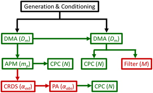
Figure 2. (a) X-ray photoelectron spectrum of a drop-cast CB thin film. Designated photoemission lines shown used for determination of elemental composition. (b) Flame ionization detector (FID) response (solid line) and temperature (dashed line) as a function of time (s) for D_m = 300 nm CB aerosol collected on a quartz filter. Temperature and atmosphere split between organic carbon (OC) and elemental carbon (EC) denoted by vertical dotted line. (c) TEM image of individual CB monomers from drop-cast aqueous suspension, scale bar is 50 nm. (d) aggregates observed from dilute suspension of CB drop-cast onto TEM grid, scale bar is 200 nm. (e) Atomized CB particles electrostatically deposited on lacey carbon grids. Scale bar represents 1 µm.

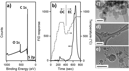
Figure 3. (a) Particle number concentration (# cm⁻³) as a function of D_m (nm) atomized from 0.25 (grey), 0.50 (blue) 1.0 (red), 2.0 (green), 4.0 (black) mg CB mL⁻¹ aqueous CB suspensions. (b) Particle mass (fg, 10⁻¹⁵ g) as a function of D_m (nm) for 0.50 (blue), 1.0 (red), 4.0 (black) mg CB mL⁻¹ aqueous CB suspensions. Dashed red line represents fit of 1.0 mg CB mL⁻¹ aqueous CB suspension using Equation (4)(4) $$Z_{\mathrm{p}}\propto \frac{q\gamma }{D_m}$$(4) . (c) Effective density (ρ_eff, g cm⁻³), calculated using Equation (5)(5) $${\rho }_{\mathrm{eff}}=\frac{6m_{\mathrm{avg}}}{\pi D_{\mathrm{m}}^3}$$(5) as a function of D_m (nm) for 0.50 (blue), 1.0 (red), 4.0 (black) mg CB mL⁻¹ aqueous CB suspensions. Dashed red line represents linear best fit of 1.0 mg CB mL⁻¹ aqueous CB suspension. Error bars are 1σ from a minimum of three measurements.

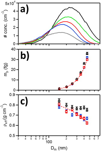
Figure 4. Measured spectroscopic data for D_m and m_p-selected CB from atomization of 1.0 mg CB mL⁻¹ aqueous CB suspensions. (a) Mass-specific absorption coefficient (MAC) as a function of wavelength for D_m = 150 nm (circles), 300 nm (squares), 450 nm (triangles) mobility, and mass selected aerosol, (b) MAC at λ = 532 nm (green) and 780 nm (black) as a function of D_m. (c) Ångström absorption exponent (AAE) using Equation (6)(6) $${\mathit{MAC}}_{\lambda }={\mathit{MAC}}_{{\lambda }_{\mathrm{REF}}}{\left(\frac{\lambda }{{\lambda }_{\mathrm{REF}}}\right)}^{-\mathrm{AAE}}$$(6) between λ = 405 nm and 780 nm as a function of D_m. (d) MAC (squares) and mass-specific extinction coefficient (MEC, circles) at λ = 405 nm (purple) and λ = 660 nm (red) as a function of D_m. (e) Single scattering albedo (SSA) at λ = 405 nm (purple triangles) and λ = 660 nm (red squares) nm as a function of D_m. Note that ordinate are identical in (a), (b), and (d). Uncertainties represent 1σ from >3 measurements and 2 production lots.

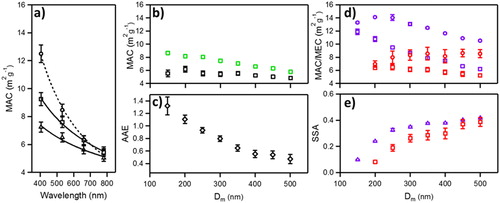
Table 1. The ensemble measured m_p and MAC_T at λ = 405 nm, 532 nm, 660 nm, and 780 nm from aqueous 1.0 mg mL⁻¹ CB suspension as a function of D_m for aerosolized CB.

Dm (nm)	mp (fg)	MACT λ = 405 nm (m^2 g^–1)	MACT λ = 532 nm (m^2 g^–1)	MACT λ = 660 nm (m^2 g^–1)	MACT λ = 780 nm (m^2 g^–1)
150	1.63 ± 0.04	12.39 ± 0.44	8.47 ± 0.77	6.36 ± 0.34	5.55 ± 0.50
200	3.59 ± 0.19	10.97 ± 0.51	8.26 ± 0.23	6.40 ± 0.27	6.18 ± 0.22
250	6.75 ± 0.32	10.00 ± 0.62	8.20 ± 0.55	6.48 ± 0.41	5.53 ± 0.37
300	11.7 ± 0.4	8.83 ± 0.58	7.60 ± 0.52	6.14 ± 0.33	5.43 ± 0.37
350	17.5 ± 0.1	8.18 ± 0.54	7.24 ± 0.38	6.11 ± 0.34	5.54 ± 0.29
400	26.0 ± 0.1	7.39 ± 0.50	6.82 ± 0.16	5.72 ± 0.32	5.23 ± 0.12
450	34.6 ± 0.3	6.91 ± 0.50	6.51 ± 0.14	5.44 ± 0.38	5.03 ± 0.11
500	48.5 ± 0.3	6.44 ± 0.49	5.81 ± 0.25	5.23 ± 0.26	4.84 ± 0.21

Uncertainty represent 1σ of multiple measurements.

Figure 5. (a) Aerosol mass concentration (M, ng m⁻³) of D_m and m_p-selected CB measured by photoacoustic spectroscopy (M_PAS) at λ = 532 nm (green circles) and 780 nm (black squares) vs. M measured by particle counting (M_C). Dashed line represents 1:1. Uncertainties in M_PAS represent propagated 1σ uncertainties in α_abs and MAC while uncertainties in M_C represent propagated 1σ uncertainties in m_p and N, respectively. We assume a 5% particle counting uncertainty across all N. (b) Filter-based mass concentration (M_F) vs. M_C of D_m = 300 nm CB using the manufacturer’s (default) MATC of 16.6 m² g⁻¹ for λ = 880 nm radiation. Dashed line represents 1:1. Uncertainties in M_F are ± 50 ng m⁻³ for filter-based measurements and for M_C the same as defined in (a). Note the order of 24× difference in M_C between (a) and (b).

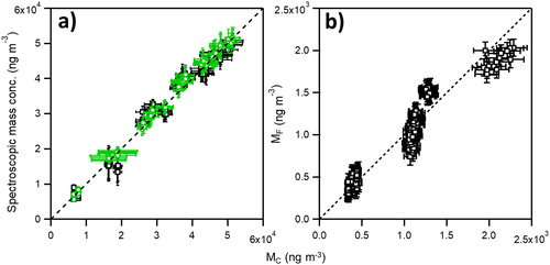
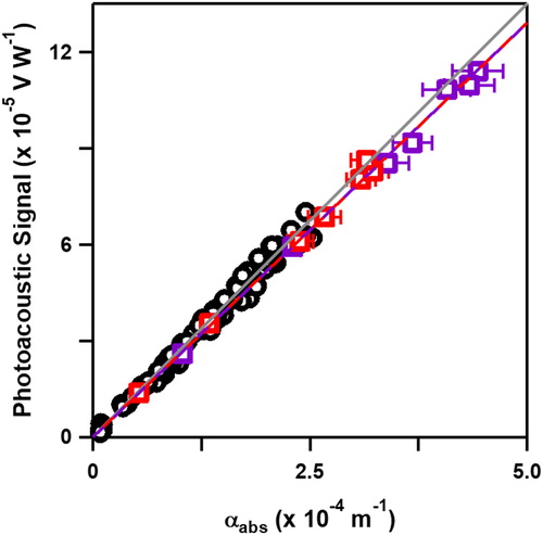
Figure 6. Photoacoustic microphone signal (V W⁻¹) as a function of α_Abs (m⁻¹) for H₂O vapor (black open circles) at λ = 725 nm and 820 nm and D_m and m_p-selected CB at λ = 405 nm (open purple squares) and λ = 660 nm (open red squares). Dashed lines are linear fits of H₂O vapor (black circles) and CB data (dashed red and purple). Uncertainties in x- and y- correspond to the standard deviations of multiple measurements and expanded uncertainties in calculated α_abs; see discussion in text.