Figures & data
Figure 1. Illustration of the three examined DC configurations. In all configurations, the resulting charge is measured with a Faraday cup electrometer (FCE). (a) Steady state (SS): corona is operated at constant voltage, (b) modulated diffusion charging (MDC): corona voltage is modulated, and (c) modulated precipitation (MP): corona is operated at constant voltage. In addition, an electrostatic precipitator is used to deposit particles depending on their electrical mobility (Schriefl, Bergmann, and Fierz Citation2019).
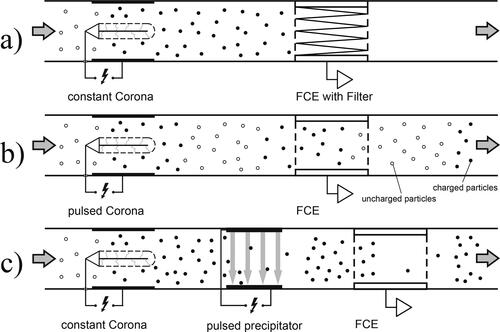
Figure 2. Schematic representation of the OpenFOAM v.5 simulation geometries representing the different stages of the modeled diffusion charger. (Illustration from Schriefl [Citation2019].)
![Figure 2. Schematic representation of the OpenFOAM v.5 simulation geometries representing the different stages of the modeled diffusion charger. (Illustration from Schriefl [Citation2019].)](/cms/asset/673458c1-3524-47f6-9b28-328a9ad5b4a5/uast_a_1873910_f0002_c.jpg)
Figure 3. Schematic of the experimental setup for the measurements of the impact of pre-charged particles on different unipolar diffusion charging configurations.
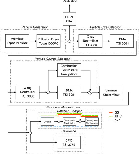
Figure 4. Charge distribution scanned with the tandem DMA setup. First DMA is set to a mobility diameter of 150 nm. Second DMA is operated in scanning mode.
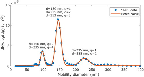
Figure 5. Mean charge curve of both simulation model and the used corona charger in the experiment. The mean charge per particle shows the mean charge acquired for the respective particle diameter. The dashed lines are linear fits through the acquired mean charges of simulation and experiment.
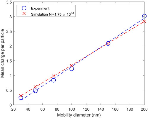
Figure 6. Counting efficiency (CE) of the three examined diffusion charging topologies. In addition to the specific number of charges, in the simulation also neutralized particle distributions (q = N) at the inlet are taken into account.
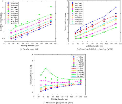
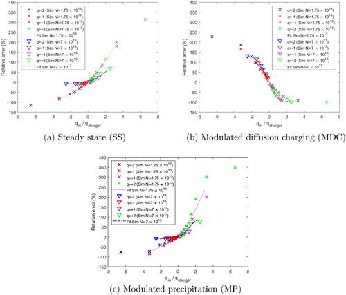
Figure 7. Relative error as a function of where
represents the mean charge at the outlet of the charger when there are no preexisting charges and
represents the mean number of preexisting charges at the inlet of the charger. Polynomial fits indicate relative error trends for simulation and experiment.
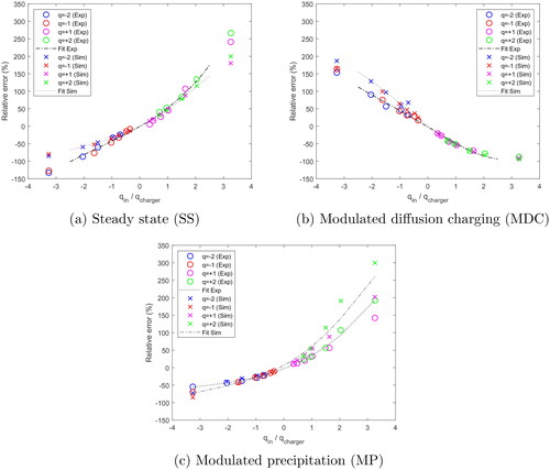
Figure 8. Simulation results for relative error as a function of Simulations are conducted with two different ion concentrations (
). Polynomial fits indicate the relative error trends for the different ion concentrations.