Identification and particle sizing of submicron mineral dust by using complex forward-scattering amplitude data

Figures & data

Figure 1. Schematic diagram of our SPES instrument with an illustration of the interferometric detection of scattered wave from each particle in forward direction.

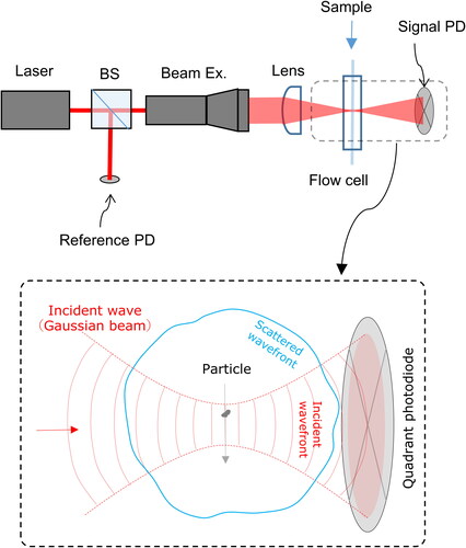
Figure 2. Scatterplot of ${{[\mathrm{Im}S}_{22}]}_{\mathrm{sc}}$ versus ${\mathrm{Re}S}_{22}$ for polystyrene spheres measured by the SPES instruments. The black dots indicate single-particle data. The red-filled circles with error bars indicate the median and 10th–90th percentile ranges of single-particle data for each particle size. The blue-filled circles with error bars indicate the theoretical values and their uncertainty ranges for each particle size. The uncertainty ranges of the theoretical values were computed from the expanded uncertainty (k = 2) of each particle size specified in the sample datasheet.

Table 1. List of samples.

Sample type	Name	Production information
Synthetic	Fullerene soot	Alfa Aesar, Inc., Stock#40971, Lot#G25N20
	Magnetite (Fe3O4)	Kojundo Chemical Laboratory Co., Ltd., FEO17PB
	Goethite (FeOOH)	Kojundo Chemical Laboratory Co., Ltd., FEI16PB
	Hematite (Fe2O3)	Kojundo Chemical Laboratory Co., Ltd., FEO14PB
	Ferrihydrite (5Fe2O3•9H2O)	Synthesized by Dr. Takahashi (Univ. of Tokyo)
	Quartz	Kojundo Chemical Laboratory Co., Ltd., SIO08PB
	Snomax®	Snomax® international
Natural	NX illite	Arginotec (NX Nanopowder, B + M Nottenkamper, Munich, Germany)
	KGa-1b	The Clay Mineral Society
	Arizona test dust (ATD)	Powder Technologies, Inc., ISOTEST DUST 12103-1, A2 fine
	Gobi dust	Environmental Certified Reference Materials No.30, National Institute for Environmental Studies, Japan.

Figure 3. Representative TEM images for each of the (a) synthetic and (b) natural samples. In (b), four elemental mappings are shown for each TEM image. The TEM images were obtained using a 120-kV TEM (JEM-1400, JEOL) and the elemental mappings were measured using an energy-dispersive X-ray spectrometer (EDS, Oxford Instruments) with scanning TEM mode (STEM-EDS).

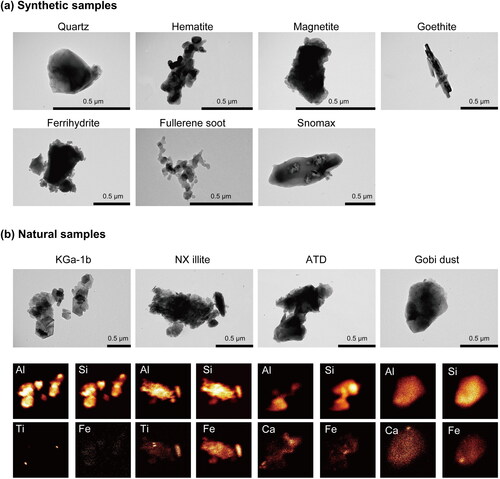
Figure 4. Scatter plots of S₂₂ data points for the individual samples listed in Table 1.

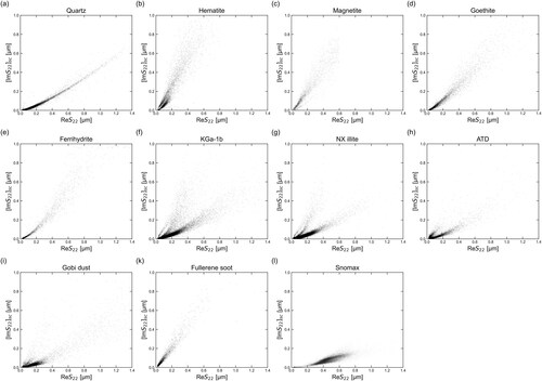
Figure 5. Density plots of $S_{22}$ data points for natural dust samples. The solid lines indicate the traces of median values of ${{[\mathrm{Im}S}_{22}]}_{\mathrm{sc}}$ as a function of ${\mathrm{Re}S}_{22}$ for each synthetic sample. Because the $S_{22}$ data points for hematite show two distinct clusters (Figure 4b), we separated the hematite data into two clusters using a boundary line (y = 0.95x – 0.02) and then computed the trace for each cluster.

Figure 6. Clustering results of $S_{22}$ data points for natural dust samples. For each sample, the (a) Boundary and (b) HDBSCAN methods were applied to the 15,000 raw data points. The black solid lines in (a) indicate the boundary curve (y = 0.65x^1.4 + 0.008). The blue solid lines with open circles indicate the principal curves for the silicate clusters, wherein the open circles indicate the 0th, 10th, …, 90th, 98th, and 100th percentiles of the arc-length coordinate of the $S_{22}$ data points. The data points with the largest 2% $\left|S_{22}\right|$ values were removed before the principal curve fitting to avoid an overfitting issue. The data number of each cluster is denoted in the legend. The total number of data points shown in each figure is less than 15,000 because of trimming of the raw data points near the origin.

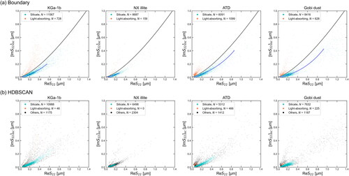
Figure 7. Bar plots of ${-\log }_{10}m(\mathit{D}|M_l)$ values for the silicate cluster. The MAP estimate of the complex refractive index m^MAP = m_r + im_i is also shown on the top of each bar plot.

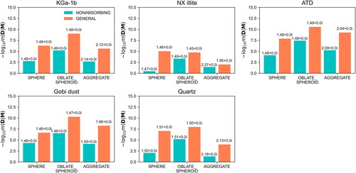
Table 2. The effective refractive indices of the silicate clusters estimated according to the Bayesian inversion method.

Sample	Refractive index	Wavelength (nm)	Method
KGa-1b	1.484 (1.461–1.497)^a	632.8	Bayesian inversion of SPES data	This study
NX illite	1.468 (1.450–1.489)^a
ATD	1.476 (1.459–1.493)^a
Gobi dust	1.463 (1.439–1.469)^a
Quartz	1.501 (1.478–1.521)^a
Kaolinite	1.556 and 1.565^b	589.6	Refractive index matching method	Weidler and Friedrich (2007)
	1.566	640	Transmission measurements	Arakawa et al. (1997)
NX Illite	1.586 and 1.588^c	589.6	Refractive index matching method	Friedrich, Steudel, and Weidler (2008)
Quartz	1.544	589.6	Refractive index matching method	Weidler and Friedrich (2007)

Note. Reported refractive index values for pure clay minerals are also shown for reference.

^a The effective refractive index is expressed as m_r^MAP along with the 10th–90th percentile range of the posterior samples of m_r.

^b Kaolinite-PW (Polwhite-B) and kaolinite-GA (Grade-A) produced by IMERYS, respectively.

^c Two test results.

Figure 8. Retrieved particle-size distributions for the silicate cluster of each dust sample. For comparison, also shown by solid lines are the retrieved particle-size distributions by elastic light scattering approaches that measure only either $\left|S_{22}\left(0°\right)\right|$ or ${\mathrm{Im}S}_{22}\left(0°\right),$ assuming m = 1.56 + 0i to be a typical refractive index value for single crystals of clay minerals.

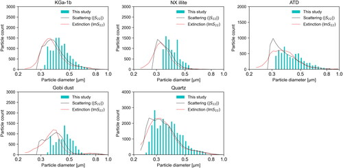
Figure B1. Scatter plots of the synthetic data that were classified by the (a) Boundary and (b) HDBSCAN methods. The black solid and black dashed lines in (a) represent the boundary curves for the curve method. Each of the blue solid lines with open circles indicates the principal curve for each silicate cluster.

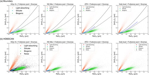
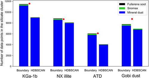
Figure B2. Number of data points in the silicate cluster for the synthetic data. Contributions to the number of data points in the silicate cluster from different components are shown. The red-filled circles indicate the original number of data points in the silicate cluster determined for each dust sample.

Weidler, P. G, and F. Friedrich. 2007. Determination of the refractive index of particles in the clay and sub-micrometer size range. Am. Mineral. 92 (7):1130–2.

 Web of Science ®Google Scholar

Arakawa, E. T. P. S. Tuminello, B. N. Khare, M. E. Millham, S. Authier, and J. Pierce. 1997. Measurement of optical properties of small particles. Oak Ridge National Lab., Oak Ridge, TN.

 Google Scholar

Friedrich, F., A. Steudel, and P. G. Weidler. 2008. Change of the refractive index of illite particles by reduction of the Fe content of the octahedral sheet. Clays Clay Miner. 56 (5):505–10.

 Web of Science ®Google Scholar