Effects of volatility, viscosity, and non-ideality on particle–particle mixing timescales of secondary organic aerosols

Figures & data

Figure 1. Schematic of the two populations implementation in KM-GAP. Both populations consist of a near-surface bulk layer (nsb) and the number of bulk layers (b_1-L; L = 10 in this study). Additionally, each particle has a sorption layer containing adsorbed and desorbing species and a near-surface gas phase to account for potential gas phase diffusion, which is not pictured. There is one shared gas phase between the two populations. Each population consists of different nonvolatile species, while population 1 initially contains semi-volatile species in equilibrium with the gas phase.

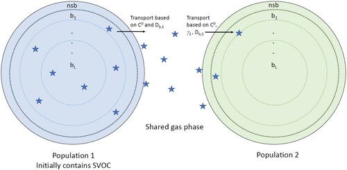
Figure 2. Particle–particle mixing timescale (τ_mix) of two populations where population 1 is liquid (D_b1 = 10⁻⁸ cm² s⁻¹) and population 2 is (a) liquid (D_b2 = 10⁻⁸ cm² s⁻¹), (b) semi-solid (D_b2 = 10⁻¹⁵ cm² s⁻¹), and (c) ultraviscous semi-solid (D_b2 = 10⁻¹⁸ cm² s⁻¹).

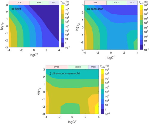
Figure 3. The final equilibrium number concentration of the semi-volatile species in population 2 with different volatilities (C⁰) and activity coefficients of semi-volatile species in population 2 (γ₂).

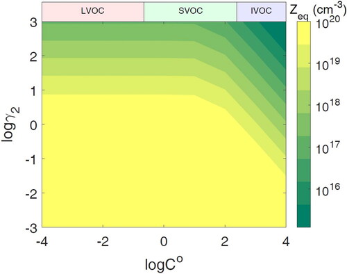
Figure 4. (a) Particle–particle mixing timescale (τ_mix) with various diffusivities and activity coefficients of semi-volatile species (C⁰ = 10 µg m⁻³) in population 2 (γ₂). (b) τ_mix when the bulk diffusivity (D_b) of a semi-volatile species with C⁰ = 10 µg m⁻³ is varied in both populations. In these simulations, the semi-volatile species is ideally miscible in both populations.

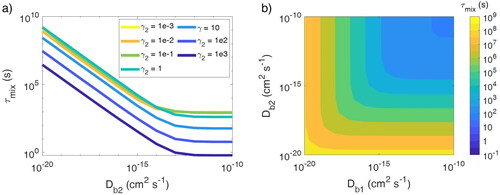
Figure 5. Particle–particle mixing timescale (τ_mix) when mass loading of population 2 (C_OA2) is varied in the range of 0.1–100 µg m⁻³, while mass loading of population 2 (C_OA1) is held constant at 40 µg m⁻³.

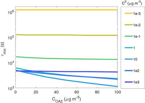
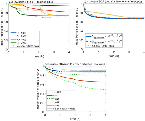
Figure 6. Simulations of toluene SOA mixing experiments and the data from Ye et al. (2016, 2018). Plotted is the mass fraction of SVOCs evaporated from population 1 in population 2. (a) Mass fraction of toluene SOA (population 1) in D-toluene SOA (population 2). RH legend indicates the RH at the end of the experiment. For each experiment, the RH begins at 10%. For RH 20%, the RH is increased at 1 h; for RH 40%, it is increased at 2 h; and for RH 90%, the experimental RH was increased continually, reaching 90% at 1 h, while in the model this is achieved by a stepwise increase in RH. (b) Mass fraction of toluene SOA (population 1) in limonene SOA (population 2) initially at 10% RH with an increase to 30% at 2 h. (c) Mass fraction of toluene SOA (population 1) in $\beta$-caryophyllene SOA (population 2) initially at 10% RH with an increase to 30% at 2 h.

Ye, Q., E. Shipley Robinson, X. Ding, P. Ye, R. C. Sullivan, and N. M. Donahue. 2016. Mixing of secondary organic aerosols versus relative humidity. Proc. Natl. Acad. Sci. USA 113 (45):12649–12654. doi: 10.1073/pnas.1604536113.

 PubMed Web of Science ®Google Scholar

Ye, Q., M. A. Upshur, E. S. Robinson, F. M. Geiger, R. C. Sullivan, R. J. Thomson, and N. M. Donahue. 2018. Following particle-particle mixing in atmospheric secondary organic aerosols by using isotopically labeled terpenes. Chem 4 (2):318–333. doi: 10.1016/j.chempr.2017.12.008.

 Web of Science ®Google Scholar