Analysis and classification of individual ambient aerosol particles with field-deployable laser-induced breakdown spectroscopy platform

Figures & data

Figure 1. The Spectroscopy Platform for Ambient Aerosol analysis (SPAA). The spectroscopy system (10.-12.) is built on a commercially available rack case and the accessory equipment (1.-8.) into an aluminum profile rack. Ambient aerosol flows through a condensation growth tube (2.) into an aerosol charger (8.) and then into the measurement chamber (10.). A virtual impactor (9.) before the chamber concentrates the grown particles and acts as a flow splitter. The lids of the rack case have not been drawn into the figure, but the depth dimension of 1.0 m is with the lids in place.

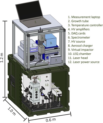
Figure 2. A schematic figure of the optical arrangement inside the chamber for single particle analysis. The aerosol is focused into the vertical axis utilizing the focusing rods. As they reach the focal spot of the lasers, the photomultiplier tube detects the scattering of the 405 nm CW laser and triggers the 355 nm pulse laser. The pulse laser turns the particle and the surrounding gas into plasma, and its emission is collected with a 19-mm focal length concave mirror. An achromatic triplet lens is utilized to focus the emission into an optical fiber bundle, which guides the emission into a 3-channel USB-spectrometer. Additionally, 2 CMOS cameras and a vertically directed 405 CW laser are utilized to monitor the focusing of the particles and the plasma-particle interaction to achieve optimal pulse laser focusing conditions.

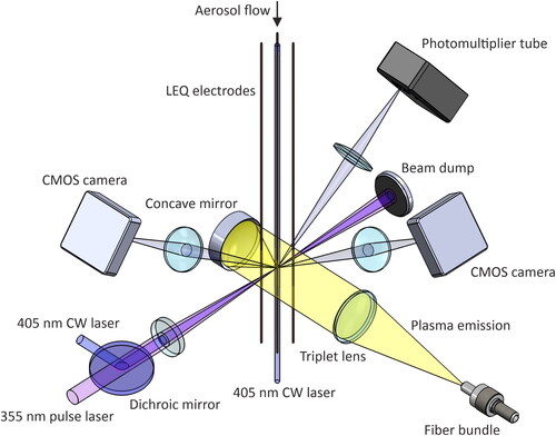
Figure 3. Emission collection optics for single-particle LIBS. The emission signal is collected with a concave mirror (f = 19 mm), focused with an achromatic triplet lens (f = 70 mm) into a fiber bundle, which is used to divide the signal into 3 spectrometers covering a wavelength range of 200–1000 nm. As the emission is collected at the focus spot of the pulse laser, the majority of the plasma emission is not seen by the spectrometer.

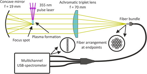
Figure 4. Measurement setup during the optimization and performance analysis experiments. Depending on the aerosol, one generation branch (Dry or Droplet generation, denoted with dashed line box) was in use at a time. After the generation, the aerosol was classified with a DMA and the particle size and concentration was monitored with an APS after classification.

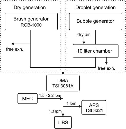
Table 1. The samples used in the resolving power analysis.

Sample no.	Mass of salt in H2O solution (g/300 ml)			Proportional mass in dry particle
	MgSO4	NaCl	KCl	Mg	Na	K
1	4.99	5.02	5.07	0.120	0.375	0.505
2	0.60	1.51	14.08	0.010	0.079	0.911
3	0.30	10.38	4.59	0.006	0.626	0.369
4	1.20	5.40	8.77	0.022	0.309	0.669

Figure 5. Results from the salt particle analysis. In panel (a), the median peak areas of the LIBS measurements are compared to the original masses of the elements in single particles. In (b), the peak areas have been calibrated using the calibration sample (1.0 µm, sample 4, Table 1) to directly estimate the mass of an element in a single particle. In (a) and (b), the mass in the horizontal axis has been calculated from the original salt solution and the particle size. In panel (c) and (d), the median values of measured fractions of mass in single particles are compared to the original values derived from the salt solutions. Error bars in all the panels indicate the IQR of either the measured or calculated values. The IQR of the original mass of the particles originates from the size distribution measured by the APS. Different colors indicate different elements and different markers indicate different particle sizes. The exceptions are the asterisk and black ‘+’ markers, which indicate the XRF and the calibration measurements, respectively. The particle size has been left out from panel (d) for clarity.

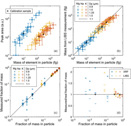
Figure 6. Results of the energy optimization measurements for Mg, Na, K, Si, and Al. Each marker represents at least 200 measurements. The energy was optimized in terms of median peak area (a) and signal variance, defined as IQR/Peak area (b).

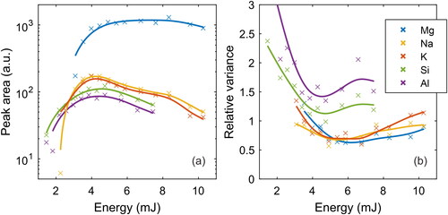
Figure 7. Example spectra from single particles acquired from generated test aerosols (a)–(b) and an average spectrum of the background measurement. The background is subtracted from each single particle spectrum.

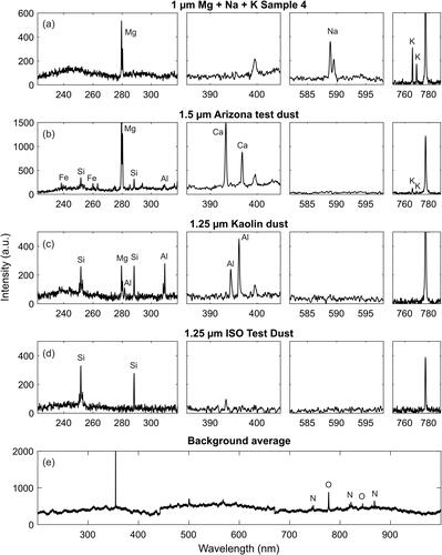
Figure 8. Example compositions calculated for the test aerosols using the Boltzmann method and NIST LIBS database normalization. Each stack of bars represents one particle, and the colors (patterns) indicate different elements. The height of a segment indicates the relative amount of an element in a particle.

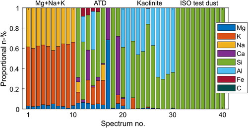
Figure 9. Normalized example compositions from the outdoors aerosol measurements. As marked into the figure, the particles are divided into four main categories due to their spectral footprints. Each bar stack represents a single particle, and the colors (patterns) indicate measured elements.

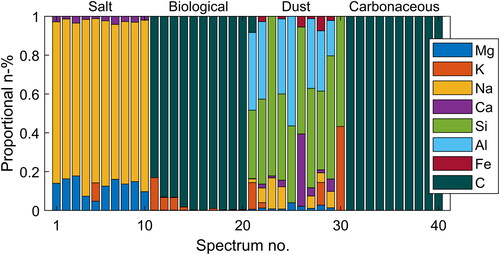
Figure 10. Example single particle spectra from the four categories of the outdoor aerosol measurement. Due to wideband operation, multiple elements could be resolved simultaneously from each particle, which enables the particle classification.

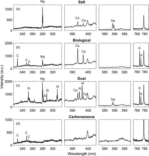
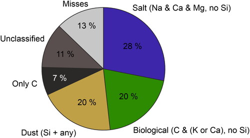
Figure 11. The relative fractions of the particle categories in the outdoor aerosol sample. Most particles were classified into the Salt category (28%), followed by Biological and Dust (20% each). 7% Included only carbon and 11% were unclassified. The unclassified particles consisted mainly of Na-rich (6%) and Ca-rich (4%) particles.

Data availability statement

All the reported data is displayed in this article.