In-situ observations of charged Saharan dust from an uncrewed aircraft system

Figures & data

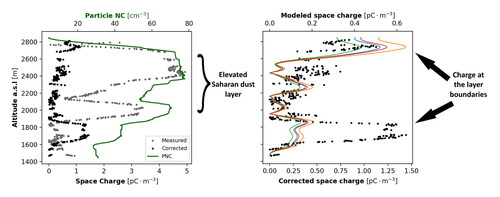
Figure 1. Single 48-h back trajectory of the sampled air mass during the day of measurements, from the HYSPLIT GDAS model (ending date time at 12:00 UTC on 6 April 2022). Three initial altitudes in m a.s.l (2500 – green, 3500 – red, and 4000 – blue line) and destination at the USRL in Orounda, Cyprus. Each colored line represents the path of the air mass with a starting altitude shown on the right and final altitude on the left, with the latter attached to a star that corresponds to the measurement location on the map. The back trajectories were similar for either flight, thus only one is shown here.

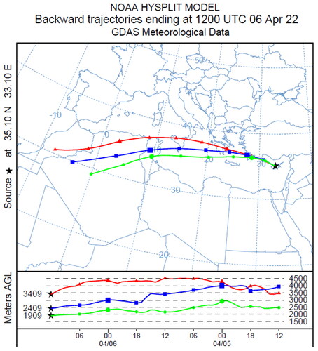
Figure 2. Images from the SEVIRI Dust RGB product on the Meteostat-8 satellite, covering two days prior to the measurement flights with the MASC-3 in Cyprus, on 6 April 2022. The images are color coded, specifically: magenta indicates dust clouds, black indicates cirrus clouds, dark red indicates ice clouds (more details on the image description can be found at EUMETSAT’s website: https://www.eumetsat.int/). The black circled areas in each image depict the first appearance and uplift of dust (upper left) on 4 April, its transport with clouds to the east through the Mediterranean (upper right and bottom left), and its arrival in Cyprus on the evening of 5 April (bottom right).

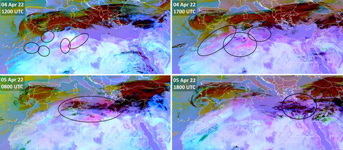
Figure 3. (a) Total attenuated backscatter at 532 nm and (b) aerosol subtype characterization, from the CALIPSO satellite, taken on 6 April at 12:24 UTC. Each plot has coordinates on the horizontal axis that cover a geographical strip that extends from North East Africa to Norway, Scandinavia (in this coordinate range, the measurement location is at: 35.095 N, 33.081 E). The satellite’s overpass was still 5–7${}^{°}$ west of Cyprus. In (a), the backscatter is color coded with the index on the side, and in (b), aerosol subtypes are also color coded and each type is denoted with a number and stated under the horizontal axis. Specifically, NA: not applicable, 1: clean marine, 2: dust, 3: polluted continental, 4: clean continental, 5: polluted dust, 6: smoke.

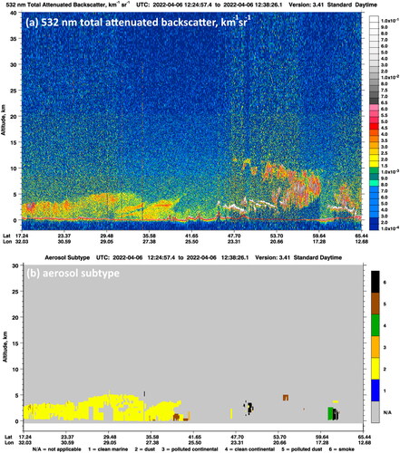
Figure 4. Volume depolarization ratio, extinction and backscatter coefficients at 532 nm wavelength, measured from the CE376 LiDAR operating in Nicosia. The profiles were captured on 6 April at 1000 UTC, at the time of the first flight of the MASC-3.

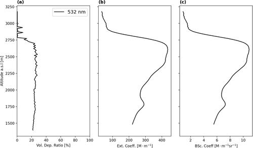
Figure 5. Vertical profiles from the two MASC-3 flights on 6 April (flight 1 at noon, flight 2 in the afternoon), showing meteorological parameters, aerosol particle number concentrations and charge sensor readings in voltages. Each row indicates a different flight. Specifically: (a) potential temperature and mixing ratio, (b) wind speed and TKE, (c) PNC (raw data and 20 s moving averaged) from 0.4 to 40 µm, and (d) charge sensor voltage as a black line, and a 10 s moving average as a red line. On the bottom row, the plots show the same parameters for the second flight, from (e) to (h). Only the ascent through the extent of the Saharan dust layer is shown in the figure.

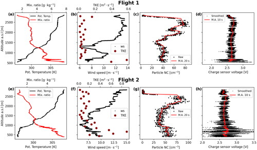
Figure 6. Aerosol particles and calculated space charge for the two flights. (a) Raw bin counts from the OPC-Pod (adding up aerosol numbers up to 1, 2.5 µm as well as the total size range of the sensor, i.e., 0.4–40 µm), (b) non-averaged PNC data in green, with a 20 s moving average as a black line, and (c) measured space charge from the Charge-Pod. On the bottom row, the plots show the same parameters for the second flight, from (d) to (f). Only the ascent is shown in the plots.

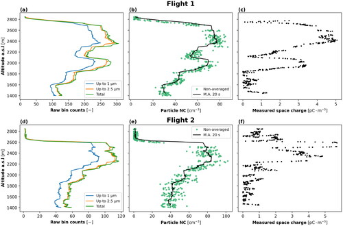
Figure 7. Scatterplot between measured particle concentrations and corresponding measured charge magnitude, covering the dust layer vertically during the MASC-3 flights. A linear fitted equation is also depicted as a red line, with the slope and intercept coefficients in the form of a line equation.

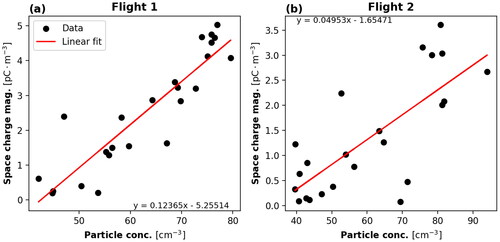
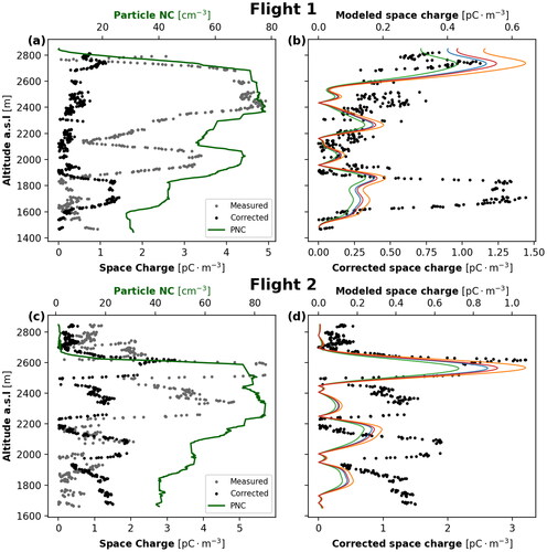
Figure 8. PNC, measured and modeled space charge, with the addition of corrected charge data, for the two flights. (a) 20 s Moving averaged PNC (green line), measured (gray points) and corrected charge (black points) on double horizontal axes, (b) modeled charge (solid lines) for different cases of background aerosol values (specifically: blue line for PNC = 1500 ${\text{cm}}^{-3}$ of 0.05 µm radius, orange line for PNC = 1500 ${\text{cm}}^{-3}$ of 0.2 µm radius, green line for PNC = 500 ${\text{cm}}^{-3}$ of 0.05 µm radius and red line for PNC = 500 ${\text{cm}}^{-3}$ of 0.2 µm radius), and corrected charge (black points) on double horizontal axes. On the bottom row, the plots show the same parameters for flight 2, from (c) to (d). Only the ascent is shown in the plots.

Data availability statement

Output of the HYSPLIT model was taken from NOAA’s website, which is available online: https://www.ready.noaa.gov. CALIPSO data were obtained from the NASA Langley Research Center Atmospheric Science Data Center: https://asdc.larc.nasa.gov/. SEVIRI data were available from Center for Environmental Data Analysis: https://data.ceda.ac.uk/badc/msg/data, and provided by EUMETSAT. AOD data were retrieved from the website of the AERONET network: https://aeronet.gsfc.nasa.gov/. Data from the UAS flights can be provided by the corresponding author, upon reasonable request.