Geophysical fluid models with simple energy backscatter: explicit flows and unbounded exponential growth

Figures & data

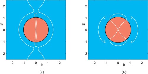
Figure 1. We plot the occurrence of explicit solutions (5(5) $\mathit{v}={\alpha }_1{\mathrm{e}}^{\lambda t}\cos (\mathit{k}\mathbf{\cdot }\mathit{x}+\tau ){\mathit{k}}^{\perp },\eta ={\alpha }_2\frac{f}{g}\sin (\mathit{k}\mathbf{\cdot }\mathit{x}+\tau )+s,$(5) ) in the plane of wave vectors with fixed parameters $d_1=1.0,b_1=1.5,b_2=2.2,f=0.3,g=9.8,H_0=0.1,{\alpha }_1=1.0$ and $d_2,{\alpha }_2$ as in the subcaptions. Red regions: $\lambda >0$, i.e. unbounded growth; blue regions: $\lambda <0$; black curves: $\lambda =0$, i.e. steady states. The white curves mark solutions with ${\alpha }_2=0$, and the white bullets mark steady solutions with $\lambda =0$. The black dashed curves mark solutions of condition (6b(6b) $\begin{array}{rl}\frac{{\alpha }_2-{\alpha }_1}{{\alpha }_1}f& =k_1{k}_2\left(\right(d_1-d_2)|\mathit{k}{|}^2+b_2-b_1),\end{array}$(6b) ) only, for ${\alpha }_2\ne 0$ with values as in the subcaptions, which also solve (6a(6a) $\begin{array}{rl}\lambda & =(b_1-d_1|\mathit{k}{|}^2)k_2^2+(b_2-d_2|\mathit{k}{|}^2)k_1^2,\end{array}$(6a) ) at the white bullets ($\lambda =0$). In (c) we mark a line of wave vectors in a fixed direction (grey), and the growing or decaying solutions (white circles) on it, whose superpositions with or without the steady state on the grey line again yield explicit solutions (Colour online).

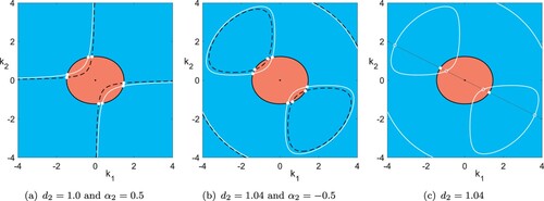
Figure 2. Possible structures of solution curves of the amplitude relation (7b(7b) $\begin{array}{rl}0& =((d_1-d_2)|\mathit{k}{|}^2+b_2-b_1)k_1{k}_2+\sigma ,\end{array}$(7b) ) analogous to figure 1. Fixed parameters: $d_1=1.0,b_1=1.5,f=0.5,g=9.8,H_0=0.1,{\alpha }_1=1.0$. It is $\sigma =0$ in (a) and $\sigma =-1$ in (b) and (c) (Colour online).

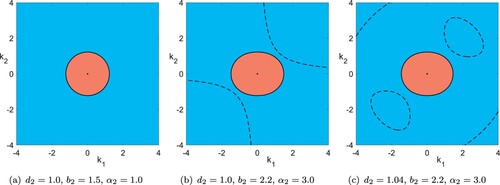
Figure 3. Solution curves (dashed lines) of the amplitude relation (7b(7b) $\begin{array}{rl}0& =((d_1-d_2)|\mathit{k}{|}^2+b_2-b_1)k_1{k}_2+\sigma ,\end{array}$(7b) ) in terms of σ, as well as their intersections with solution curves of the dispersion relation (7a(7a) $\begin{array}{rl}\lambda & =-(d_1{k}_2^2+d_2{k}_1^2)|\mathit{k}{|}^2+b_1{k}_2^2+b_2{k}_1^2,\end{array}$(7a) ) with $\lambda =0$; the grey lines mark $k_2=m{k}_1$. Denotations as in figure 1 with focus on upper left quadrant. In (a) there are no explicit solutions. In (b) and (c) steady solution occur at intersection point (white dot). Fixed parameters: $d_1=1.0,d_2=1.0,b_1=1.5,b_2=2.2,f=0.3,g=9.8,H_0=0.1,{\alpha }_1=1.0$ (Colour online).

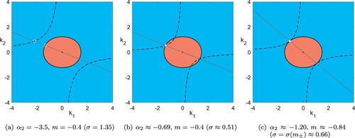
Figure 4. Information on the spectrum of the linearisation of (1(1a) $\begin{array}{rl}\frac{\mathrm{\partial }\mathit{v}}{\mathrm{\partial }t}+(\mathit{v}\mathbf{\cdot }\mathbf{\nabla })\mathit{v}& =-f{\mathit{v}}^{\perp }-g\mathbf{\nabla }\eta -\left(\begin{array}{cc}{d}_1{\mathrm{\Delta }}^2+b_1\mathrm{\Delta }& 0\\ 0& d_2{\mathrm{\Delta }}^2+b_2\mathrm{\Delta }\end{array}\right)\mathit{v},\end{array}$(1a) ) in the trivial steady solution $({\mathit{v}}_s,{\eta }_s)\equiv (0,0,0)$ for parameters $d_1=1.0,d_2=1.04,b_1=1.5,b_2=2.2,f=-0.3,g=9.8,H_0=0.1$. (a) Signs of the most unstable real part of elements in the spectrum in terms of the wave vector $\mathit{k}$ of the associated eigenmodes – real part positive (red region), negative (blue region); black dot and curve correspond to steady states of (5(5) $\mathit{v}={\alpha }_1{\mathrm{e}}^{\lambda t}\cos (\mathit{k}\mathbf{\cdot }\mathit{x}+\tau ){\mathit{k}}^{\perp },\eta ={\alpha }_2\frac{f}{g}\sin (\mathit{k}\mathbf{\cdot }\mathit{x}+\tau )+s,$(5) ). Note the unstable non-real spectrum in addition to, e.g. figure 1. (b) The real part of the spectrum for $k_2=0$, showing unstable spectrum in the vicinity of the origin (Colour online).

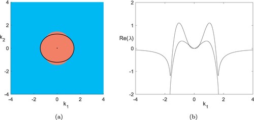
Figure 5. Examples for unboundedly unstable explicit steady solutions (5(5) $\mathit{v}={\alpha }_1{\mathrm{e}}^{\lambda t}\cos (\mathit{k}\mathbf{\cdot }\mathit{x}+\tau ){\mathit{k}}^{\perp },\eta ={\alpha }_2\frac{f}{g}\sin (\mathit{k}\mathbf{\cdot }\mathit{x}+\tau )+s,$(5) ) for the same parameter values as in figure 1(c). (a) Red arcs mark unboundedly unstable steady solutions. Grey curves mark explicit time-dependent solutions with ${\alpha }_2=0$. (b) Graph of $\sigma \left(\phi \right)$. Red parts mark unboundedly unstable cases; dashed grey line marks the value of the Coriolis parameter f (Colour online).

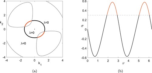
Figure 6. Illustration of long-wavelength instabilities of explicit flows. (a and b) Wave vectors $\mathit{k}=|\mathit{k}|(\cos \phi ,\sin \phi {)}^{\mathsf{T}}$ of explicit solutions (5(5) $\mathit{v}={\alpha }_1{\mathrm{e}}^{\lambda t}\cos (\mathit{k}\mathbf{\cdot }\mathit{x}+\tau ){\mathit{k}}^{\perp },\eta ={\alpha }_2\frac{f}{g}\sin (\mathit{k}\mathbf{\cdot }\mathit{x}+\tau )+s,$(5) ) as functions of φ. Black: steady solutions ${\mathit{k}}_s\left(\phi \right)$; blue: exponentially decaying; red: exponentially growing. (c) Growth rate λ as a function of the difference of wave vector lengths from steady solution. Parameters for all three cases as in figure 1(c) (Colour online).

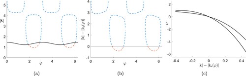
Figure 7. Shown are the eigenvalues with real part larger than $-0.1$ of an approximation of ${\mathbf{L}}_1$ with N = 10 wave modes, i.e. $3(2N+1{)}^2$ Fourier modes on the periodic domain $[0,2\pi /k_1]\times [0,2\pi /k_2]$, and Bloch modes from the grid with distance $\pi /4$. Parameters are as in figure 1(c) and s = 0. Amplitudes are ${\alpha }_1=1$ and ${\alpha }_2=0$, so $\sigma =f=0.3$ and the selected steady solution corresponds to the point between the red and black arcs in figure 5 with $\mathit{k}\approx (-1.4,0.35)$. In particular, the solution is already unstable at marginal instability with respect to the explicit modes.

Figure 8. Signs of λ as defined in the dispersion relation (25a(25a) $\begin{array}{rl}{\lambda }_i& =(b_1-d_1{s}^2)k_{i,2}^2+(b_2-d_2{s}^2)k_{i,1}^2,\end{array}$(25a) ) (red: $\lambda >0$, blue: $\lambda <0$, black: $\lambda =0$) and possible wave vectors for (24(24a) $\begin{array}{rl}\mathit{v}(t,\mathit{x})& =\sum _{i=1}^N{\mathrm{e}}^{{\lambda }_{i}t}{\psi }_i{\mathit{k}}_i^{\perp }\text{with}{\psi }_i={\alpha }_i\sin ({\mathit{k}}_i\mathbf{\cdot }\mathit{x}+{\tau }_i),1\le i\le N,\end{array}$(24a) ) for a fixed wave number s>0 (white circles). White dots mark wave vectors of corresponding steady solutions. Fixed parameters are $d_1=1.0,d_2=1.04,b_1=1.1,b_2=2.2$, i.e. $b_1/d_1\ne b_2/d_2$ (Colour online).

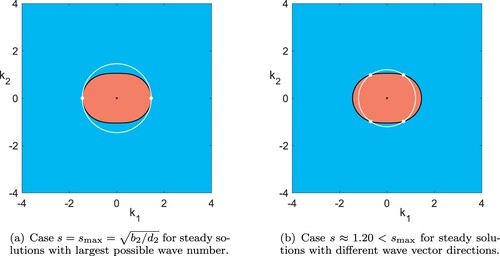
Figure 9. Shown is an approximation of part of the spectrum of ${\tilde{\mathit{L}}}_1$. Using (30(30) $({\tilde{\mathit{L}}}_1\mathit{v}{)}_m=({\mathbf{L}}_1\mathit{v}{)}_m-\frac{{\mathit{k}}_m\mathbf{\cdot }({\mathbf{L}}_1\mathit{v}{)}_m}{|{\mathit{k}}_m{|}^2}{\mathit{k}}_m=(\mathsf{I}-\mathsf{B}\left({\mathit{k}}_m\right))({\mathbf{L}}_1\mathit{v}{)}_m,$(30) ) we reduced to two-dimensional wave vectors by fixing the third component of ${\mathit{k}}_m$ at zero. Here, $\mathit{k}=(1,1)$, ${\alpha }_1=0.1,{\alpha }_2=1$. As in figure 7 we use N = 10 wave modes, i.e. $3(2N+1{)}^2$ Fourier modes on the periodic domain $[0,2\pi /k_1]\times [0,2\pi /k_2]$, and Bloch modes in the first component from the grid with distance $\pi /8$. In particular, the spectrum is unstable, so that large amplitude solutions are linear unstable with growth rates proportional to the amplitude.

Figure 10. Unboundedly growing Kolmogorov flows occur for wave vectors $(k,m)$ in the red regions for parameter sets $\mathrm{\Lambda }:=\{N^2,d_1,b_1,d_2,b_2,d_3,b_3,\mu \}$ (with isotropic backscatter), where the Coriolis parameter is fixed at f = 1. Red regions: one of conditions (i), (ii) and (iii) is satisfied; blue regions: none of conditions (i), (ii) and (iii) is satisfied; black curves in (a): loci of $c_0=c_1=c_2=0$; black curves in (b–e): loci of $c_0=0$; white dots: the zero state at $(k,m)=(0,0)$ (Colour online).

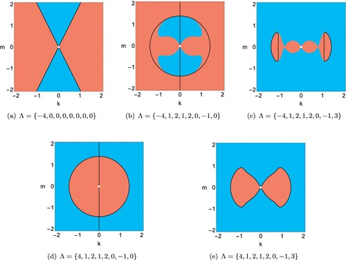
Figure 11. Existence of MGW solutions on the wave vector plane $(k,m)$ in the case $\omega ,{\alpha }_1\ne 0$ (white curves) with growth rate λ positive (red), zero (black) or negative (blue). Fixed parameter: $d_1=0.12,d_3=0.0,b_1=0.14,b_3=-0.1,\mu =0.12,f=0.3$. (a) Stable stratification $N^2=1$ with anisotropic backscatter $d_2=0.11,b_2=0.12$. (b) Unstable stratification $N^2=-0.05$ with isotropic backscatter $d_2=0.12,b_2=0.14$ (Colour online).