Modeling Watershed-Scale Historic Change in the Alpine Treeline Ecotone Using Random Forest

Figures & data

Figure 1. Observation extents in the West Castle Watershed (WCW); (a) elevation gradient in the WCW, with crosshatched shading showing areas that were visible in Mountain Legacy Project (MLP) imagery, (b) SPOT 6 RGB image of the WCW, 150 cm resolution, captured 31 July 2014, copyright 2014 CNES – shaded areas show the Alpine Treeline Ecotone (ATE) region of the watershed, 1700–2200 m a.s.l.

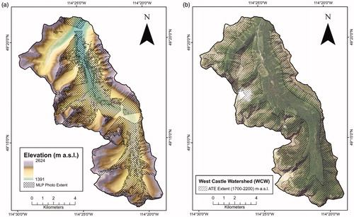
Figure 2. Image classification workflow, adapted from McCaffrey and Hopkinson (2017); (a) an oblique image of Mount Haig, in the West Castle Watershed (WCW); (b) a 20 m fishnet applied to the orthogonal Mount Haig view shed; (c) fish net grid projected back to oblique view using WSL monoplotting tool; (d) oblique image with ordinal canopy cover classification, red = no cover, yellow = low vegetation, light green = partial canopy, dark green = full canopy; (e) orthogonal image with canopy cover classification; (f) change class for Alpine Treeline Ecotone (ATE) elevation (1700–2200 m a.s.l.), red = vegetation decrease, beige = no change, green = vegetation increase. Background images in a, c, and d copyright Mountain Legacy Project 2016, and in b, e, f, copyright CNES 2014.

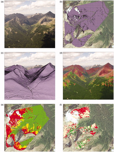
Figure 3. Canopy change classification for area observed in Mountain Legacy Project (MLP) imagery, at Alpine Treeline Ecotone (ATE) elevation. Areas of vegetation decrease, in red, occur predominantly on warm slopes, while areas of vegetation decrease, in green, occur on cool slopes.

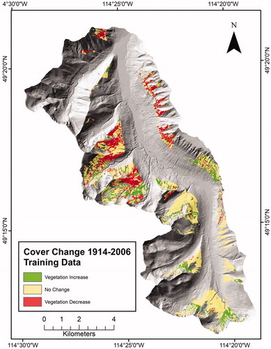
Figure 4. Variables used in random forest model training; (a) elevation, (b) compound topographic index (CTI), (c) curvature, (d) slope, (e) annual solar radiation, (f) aspect, (g) fire occurrence, (h) surficial geology; and model validation, (i) fractional cover.

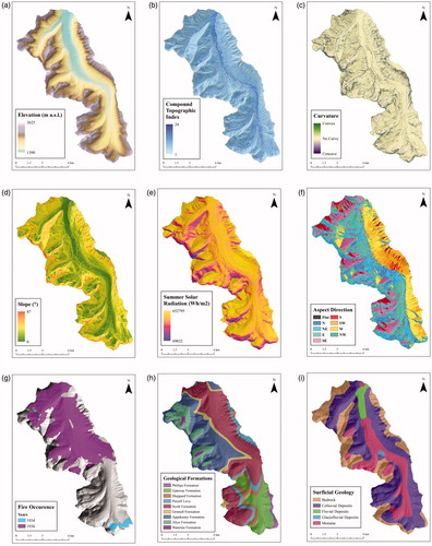
Table 1. Summary of continuous variables used in random forest model.

		Mean		Std dev.		Max		Min
Variable	Unit	Training	Prediction	Training	Prediction	Training	Prediction	Training	Prediction
Elevation	m a.s.l.	1878.77	1957.35	134.24	136.75	2199.78	2199.99	1700.23	1700.02
Compound topographic index	Unitless	5.43	5.64	1.23	1.80	12.06	18.42	2.98	1.47
Curvature	Unitless	0.11	−0.11	1.10	2.51	9.42	69.99	−10.53	−62.62
Slope	°	29.87	30.04	8.80	12.55	67.76	87.38	2.43	0.01
Annual precipitation	mm	1518.98	1582.57	142.12	157.63	1858.28	1936.46	1211.33	1195.98
Annual solar radiation	Wh/m2	1,231,776.75	1,092,610.75	145,166.80	265,128.56	1,478,222.13	150,9141.88	709,934.25	171,480.11
Annual temperature	°C	1.87	1.51	0.59	0.60	2.84	2.95	0.30	−0.03
Summer PET	mm/day	1.33	1.22	0.09	0.23	1.51	1.52	0.95	0.17
Summer precipitation	mm	259.23	270.04	17.51	17.97	301.13	305.14	235.59	234.99
Summer solar radiation	Wh/m2	539,345.31	499,860.88	37,075.29	91,860.95	627,617.13	626,085.31	369,672.28	70,528.40
Summer temperature	°C	10.79	10.52	0.54	0.56	11.52	11.73	9.48	9.45

Training indicates values within observed ATE area of the WCW, prediction indicates values in unobserved ATE area.

Table 2. Summary of categorical variables used in random forest model.

	Observed		Predicted
Variable	Count	Percent	Count	Percent
Aspect
N	7018	16.0	8232	8.7
NE	7172	16.4	10460	11.1
E	8803	20.1	13870	14.7
SE	5916	13.5	19448	20.5
S	1943	4.4	7154	7.6
SW	4862	11.1	9598	10.1
W	3782	8.6	15253	16.1
NW	4241	9.7	10625	11.2
Fire exposure
Fire	21158	48.4	59927	63.3
No fire	22580	51.6	34713	36.7
Surficial geography
Colluvial deposit	26635	60.9	51737	54.7
Moraine	7522	17.2	10104	10.7
Bedrock	9581	21.9	32711	34.6

Percentages are among group, within observed and unobserved condition.

Table 3. Confusion matrix for vegetation change classes, with overall accuracy, precision, recall, and Cohen’s Kappa scores.

	Predicted
Observed	Veg. decrease	No change	Veg. increase	Row total	Recall
Veg. decrease	1340	538	59	1937	0.69
No change	372	4716	281	5369	0.88
Veg. increase	90	649	703	1442	0.49
Column total	1802	5903	1043	Overall Accuracy = 0.77
Precision	0.74	0.80	0.67	Cohen's Kappa = 0.56

Figure 5. Predicted Alpine Treeline Ecotone (ATE) canopy change classification in areas of the West Castle Watershed (WCW) that were unobserved in Mountain Legacy Project (MLP) imagery. Predictions were also provided for observed areas, which are labeled as training areas (shaded). Vegetation decrease is generally predicted on warm, fire-exposed aspects, and vegetation increase is predicted on cool, non-fire exposed aspects.

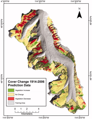
Figure 6. Boxplots of LiDAR-derived fractional cover measurements, comparing Alpine Treeline Ecotone (ATE) canopy cover change classifications. On the left, observed change classes, and on the right, change classes predicted in the random forest model. In both conditions, fractional cover in the vegetation increase class is significantly higher than the in the vegetation decrease class.

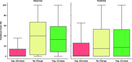
Figure 7. Boxplot showing permutation importance for the 21 variables used in the initial model accuracy assessment. Great accuracy reduction is associated with higher importance, as the model loses more accuracy when these variables are permuted. PET: Potential Evapotranspiration; CTI: Compound Topographic Index.

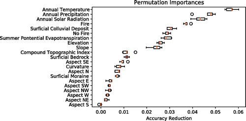
Figure 8. Pearson correlation matrix for the continuous model variables. PET: Potential Evapotranspiration; CTI: Compound Topographic Index.

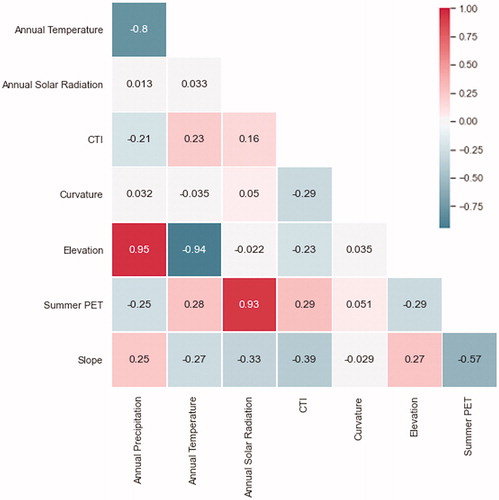
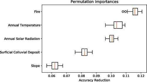
Figure 9. Boxplot showing permutation importance for the five model variables selected by the recursive feature elimination algorithm.

McCaffrey, D.R., and Hopkinson, C. 2017. “Assessing fractional cover in the alpine treeline ecotone using the WSL monoplotting tool and airborne LiDAR.” Canadian Journal of Remote Sensing, Vol. 43(No. 5): pp. 504–512.

 Web of Science ®Google Scholar