Synthetic magnetotelluric modelling of a regional fault network – implications for survey design and interpretation

Figures & data

Figure 1. 3D perspective view of the fault model used for synthetic inversion. Faults are shown in green. Diagram is shown on an equal horizontal and vertical scale.

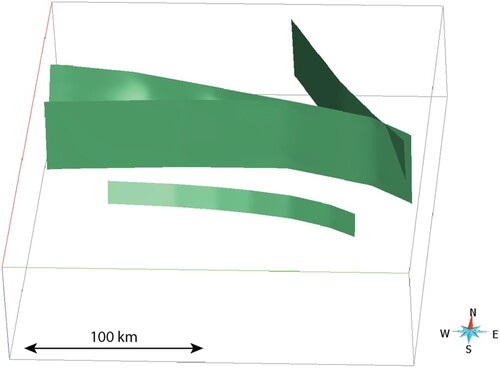
Figure 2. Synthetic model setup for calculating the forward responses, at 2 and 20 km depth. (a–b) example with a thicker, more conductive fault (750 m model cell size, Scenario 1), (c–d) example with a thinner, less conductive fault (500 m model cell size, Scenario 2). Black circles indicate sites on a ∼55 km grid, crosses indicate sites added for a ∼28 km densification around the faults, plus symbols indicate sites added for a ∼14 km densification in a N-S direction, and dots indicate sites added for a ∼7 km densification in a N-S direction.

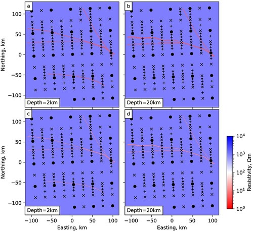
Table 1. Mesh parameters used for inversion of synthetic data.

Station spacing (°)	Min station spacing N-S (km)	Min station spacing E-W (km)	Horizontal cell size (km)	Number of vertical cells	Vertical cell size at 40 km depth (km)	RMS misfit (Scenario 1)	RMS misfit (Scenario 2)	RMS misfit (Scenario 3)
0.5	55	47	10	120	1.4	2.14	1.74	2.47
0.25	28	24	6	120	1.4	1.85	1.60	1.75
0.125	14	24	3	120	1.4	1.71	1.49	1.91
0.0625	6.9	24	1.5	120	1.4	1.69	1.87	1.66
0.5	55	47	10	30	10.5	2.25
0.25	28	24	6	40	6.7	1.89
0.125	14	24	3	60	3.5	1.70

Figure 3. Depth slices at 2 km showing inverted resistivity from progressively densified MT arrays with minimum station spacing of ∼55 km (0.5°), ∼28 km (0.25°), ∼14 km (0.125°), and ∼7 km (0.0625°). Top panel (a–d) shows Scenario 1 (750–1500 m wide fault, 5 Ωm, Figure 2 (a and b)); middle panel (e-h) shows Scenario 2 (500–1000 m wide fault, 10 Ωm, Figure 2 (c and d)), bottom panel (i–l) shows Scenario 3 (same as Scenario 1 but all sites on even 0.5 degree (∼55 km) intervals of latitude and longitude were inverted with only long-period data). Stations with short-period data (>0.001 s) are shown as dots, stations with only longer-period data (>10 s) are shown as crosses.

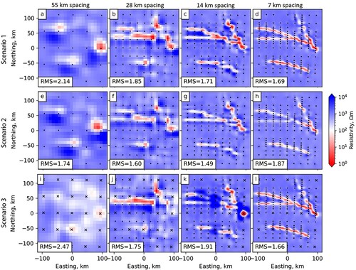
Figure 4. Depth slices at 20 km showing inverted resistivity from progressively densified MT arrays with minimum station spacing of ∼55 km (0.5°), ∼28 km (0.25°), ∼14 km (0.125°), and ∼7 km (0.0625°). Top panel (a–d) shows Scenario 1 (750–1500 m wide fault, 5 Ωm, Figure 2 (a and b)); middle panel (e–h) shows Scenario 2 (500–1000 m wide fault, 10 Ωm, Figure 2 (c and d)); bottom panel (i–l) shows Scenario 3 (same as Scenario 1 but all sites on even 0.5 degree (∼55 km) intervals of latitude and longitude were inverted with only long-period data). Stations with short-period data (>0.001 s) are shown as dots, stations with only longer-period data (>10 s) are shown as crosses.

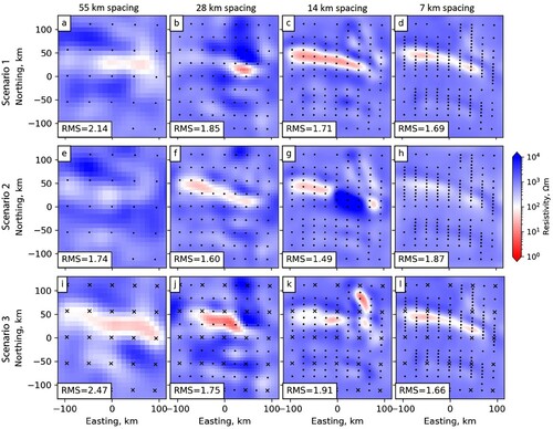
Figure 5. North-south section through the centre of the model for Scenario 1 (0 km E) showing the inversions from progressively densified data with spacing equal to ∼55 km (0.5°; top panel), ∼28 km (0.25°; second panel), ∼14 km (0.125°; third panel), and ∼ 7 km (0.0625°; bottom left panel). Bottom right panel (h) shows the true model. Left panel (a, c, e and g) shows the main inversions as presented in Figure 3, while b, d, f show models with a coarser vertical mesh (text and Table 1).

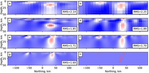
Figure A1. Depth slices at 10 km showing inverted resistivity from progressively densified MT arrays with minimum station spacing of 0.5, 0.25, 0.125, and 0.0625 degrees of latitude/longitude (approximately 55, 28, 14 and 7 km). Top panel (a–d) shows Scenario 1 (750–1500 m wide fault, 5 Ωm, Figure 2 (a and b) of main manuscript); middle panel (e–h) shows Scenario 2 (500–1000 m wide fault, 10 Ωm, Figure 2 (c and d) of main manuscript); bottom panel (i–l) shows Scenario 3 (same as Scenario 1 but all sites on even 0.5 degree (∼55 km) intervals of latitude and longitude were inverted with only long-period data). Stations with short-period data (>0.001 s) are shown as dots, stations with only long-period data (>10 s) are shown as crosses.

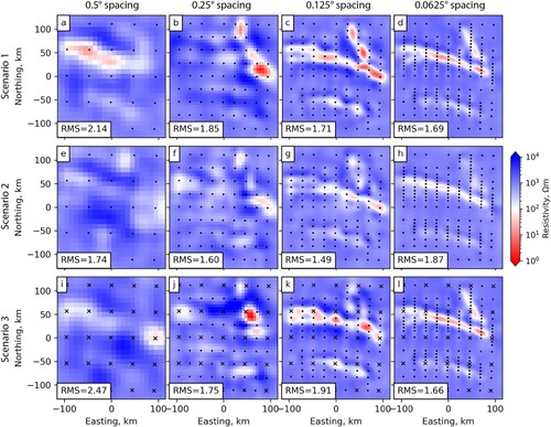
Figure A2. North–south section at −50 km E showing inversions from Scenario 1 and Scenario 1 with a coarser vertical mesh using progressively densified data arrays with spacing across strike equal to ∼55 km (0.5°; top panel), ∼28 km (0.25°; second panel), ∼14 km (0.125°; third panel), and ∼ 7 km (0.0625°; bottom left panel). Bottom right panel (h) shows the true model. Left panel (a, c, e and g) shows the main inversions as presented in Figure 3 of the main manuscript, b, d, f shows models with a coarser vertical mesh (main manuscript text and Table 1).

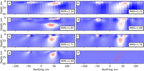
Figure A3. North-south section at 0 km E showing inversions from Scenario 1 and Scenario 1 with a coarser vertical mesh using progressively densified data arrays with spacing across strike equal to ∼55 km (0.5°; top panel), ∼28 km (0.25°; second panel), ∼14 km (0.125°; third panel), and ∼ 7 km (0.0625°; bottom left panel) . Bottom right panel (h) shows the true model. Left panel (a, c, e and g) shows the main inversions as presented in Figure 3 of the main manuscript, b, d, f shows models with a coarser vertical mesh (main manuscript text and Table 1).

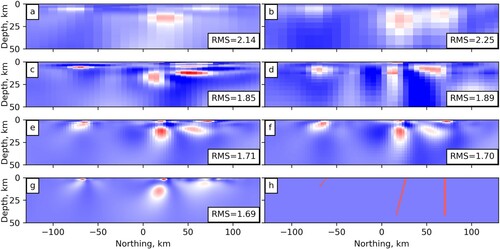
Figure A4. North-south section at 0 km E showing inversions from Scenarios 2 and 3 using progressively densified data arrays with spacing across strike equal to ∼55 km (0.5°; top panel), ∼28 km (0.25°; second panel), ∼14 km (0.125°; third panel), and ∼ 7 km (0.0625°; bottom panel). Left panel (a, c, e and g) shows Scenario 2 discussed in the main text with the narrower, less conductive fault zone setup; b, d, f and h show Scenario 3 (see main manuscript text and Table 1 for further details).

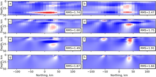
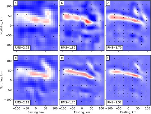
Figure A5. Depth slices at 2 km showing inverted resistivity from the synthetic data of Scenario 1 (coarse vertical mesh) in the main text, with a covariance of 0.6 as used in the main text (top panel) and 0.3 (bottom panel). Minimum station spacing of (a and d) ∼55 km (0.5°); (b and e) ∼28 km (0.25°); and (c and f) ∼14 km (0.125°).

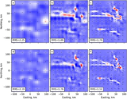
Figure A6. Depth slices at 10 km showing inverted resistivity from Scenario 1 (coarse vertical mesh) in the main text, with a covariance of 0.6 as used in the main text (top panel) and 0.3 (bottom panel). Minimum station spacing of (a and d) ∼55 km (0.5°); (b and e) ∼28 km (0.25°); and (c and f) ∼14 km (0.125°).

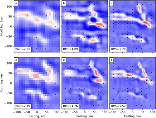
Figure A7. Depth slices at 20 km showing inverted resistivity from Scenario 1 (coarse vertical mesh) in the main text, with a covariance of 0.6 as used in the main text (top panel) and 0.3 (bottom panel). Minimum station spacing of (a and d) ∼55 km (0.5°); (b and e) ∼28 km (0.25°); and (c and f) ∼14 km (0.125°).