Towards an absolute scale for adhesion strength of ship hull microfouling

Figures & data

Figure 1. Geometry and boundary conditions: (a) schematic representation of a vertically impinging jet; (b) boundary conditions for axisymmetric cases simulated in the present study, where the symmetry axis coincides with the x axis. The drawings are not to scale.

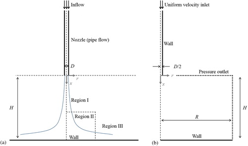
Table 1. Previous experimental and numerical studies on vertically impinging circular jets.

Reference	H/D	Re	Technique for wall shear stress	Nozzle type
Bradshaw & Love (1961)	18	1.5 × 10^5	Flat Preston tube (air)	Pipe
Poreh, Tsuei, and Cermak (1967)	8–24	1.11 × 10^6–5.00 × 10^6	Floating element (air)	Orifice
Kataoka & Mizushina (1974)	3.86–8.24	9.60 × 10^3–3.62 × 10^4	Electro-chemical (water)	Convergent
Beltaos & Rajaratnam (1974)	21.2–65.7	3.89 × 10^4–8.04 × 10^4	Preston tube (air)	Convergent
Giralt, Chia, and Trass (1977)	3.0–25.0	3 × 10^4–8 × 10^4	Not determined (air)	Convergent
Hanson, Robinson, and Temple (1990)	16.5	2.3 × 10^4–8.4 × 10^4	Hot-film sensor (water)	Convergent
Alekseenko & Markovich (1994)	2–8	4.16 × 10^4	Electrochemical (water)	Convergent
Phares, Smedley, and Flagan (2000)	3–20	3.7 × 10^3–1.15 × 10^4	Particle resuspension (air)	Short pipe
Shademan, Balachandar, and Barron (2013)	2–18.5	1 × 10^5	RANS	Uniform inlet
Ghaneeizad, Atkinson, and Bennett (2015)	24.7	2.3 × 10^4–3.4 × 10^4	PIV (water)	JET nozzle
Shademan et al. (2016)	20	2.8 × 10^4	LES, PIV (water)	Convergent

RANS, Reynolds-averaged Navier–Stokes; LES, large eddy simulation; PIV, particle image velocimetry; JET, jet erosion test.

Table 2. Flow cases simulated in this study, where H/D = 20 is used throughout.

D [m]	Re	u0 [m s^−1]	Purpose
0.01	28,000	2.811	Validation (Shademan et al. 2016)
0.0016	7,000	4.4	Empirical study on scaling parameters (adhesion testing)
	18,000	11.3
	29,000	18.2
	40,000	25.1

Figure 2. Axisymmetric grids used in this study (coarse grids): (a) grid A1, and (b) grid B1. All grid cells are represented.

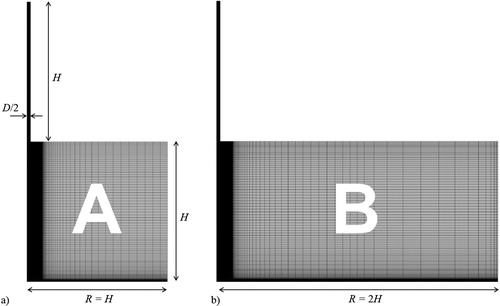
Table 3. Grid convergence index (GCI) for the fine grid solution (stagnation pressure p_s and maximum wall shear stress τ_w,max), calculated according to Equation 6(6) $$\mathit{GCI}\mathrm{ }\left[\text{fine grid}\right]=3\mathrm{ }\left|\left|\frac{f_1-f_2}{f_2}\right|\right|/({\mathit{Gr}}^{\mathit{Np}}-1)$$(6) , based on Roache (1994), for the validation case (D = 0.01 m, Re = 28,000).

Turbulence model and domain size	ps [Pa]			τw,max [Pa]
	f1	f2	GCI	f1	f2	GCI
SST, grid A	456	446	2.2%	6.13	6.22	1.3%
SST, grid B	455	445	2.1%	6.12	6.21	1.4%
ReaKEps, grid A	399	413	3.3%	4.40	4.51	2.4%
ReaKEps, grid B	399	404	1.3%	4.40	4.45	1.2%

Figure 3. Centreline velocity $\overline{u}$/u₀ along the axial length x/D. This study: ▬ ▬ (red) SST Grid A1, ▬ (red) SST Grid A2, ▬ ▬ (black) SST Grid B1, ▬ (black) SST Grid B2, ▬ ▬ (green) ReaKEps Grid A1, ▬ (green) ReaKEps Grid A2, ▬ ▬ (blue) ReaKEps Grid B1, ▬ (blue) ReaKEps Grid B2. Reference experimental studies: –♦– H/D = ∞ (Giralt, Chia, and Trass 1977), △ H/D = 22.0 (Giralt, Chia, and Trass 1977), –○– H/D = 20 (Shademan et al. 2016), ■ H/D = 15.56 (Giralt, Chia, and Trass 1977). Note that results for grids A and B practically overlap.

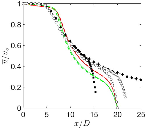
Figure 4. Radial velocity $\overline{v}$/u₀, at four radial distances, for a) SST model, b) ReaKEps model. This study: ▬ ▬ (red) SST Grid A1, ▬ (red) SST Grid A2, ▬ ▬ (black) SST Grid B1, ▬ (black) SST Grid B2, ▬ ▬ (green) ReaKEps Grid A1, ▬ (green) ReaKEps Grid A2, ▬ ▬ (blue) ReaKEps Grid B1, ▬ (blue) ReaKEps Grid B2. Reference experimental study: ◊ r/D = 0, △ r/D = 1, ■ r/D = 2, × r/D = 3 (Shademan et al. 2016). Note that results for grids A and B practically overlap.

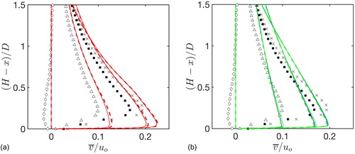
Figure 5. Wall pressure p/p_s as a function of radial distance r/r_1/2. This study: ▬ ▬ (red) SST Grid A1, ▬ (red) SST Grid A2, ▬ ▬ (black) SST Grid B1, ▬ (black) SST Grid B2, ▬ ▬ (green) ReaKEps Grid A1, ▬ (green) ReaKEps Grid A2, ▬ ▬ (blue) ReaKEps Grid B1, ▬ (blue) ReaKEps Grid B2. Reference studies: ▬ Beltaos & Rajaratnam (1974) (experimental), ○ Shademan, Balachandar, and Barron (2013) (RANS). Note that results for grids A and B practically overlap.

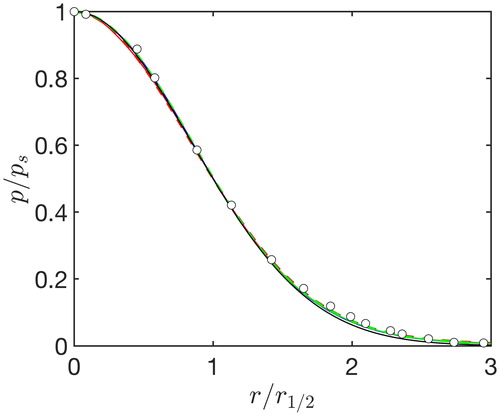
Figure 6. Dimensionless wall shear stress as a function of radial distance. This study: ▬ ▬ (red) SST Grid A1, ▬ (red) SST Grid A2, ▬ ▬ (black) SST Grid B1, ▬ (black) SST Grid B2, ▬ ▬ (green) ReaKEps Grid A1, ▬ (green) ReaKEps Grid A2, ▬ ▬ (blue) ReaKEps Grid B1, ▬ (blue) ReaKEps Grid B2. Reference studies: –□– H/D = 18, experimental (Bradshaw & Love 1961), –◊– H/D = 21.2, experimental (Beltaos & Rajaratnam 1974), * H/D = 16.5, experimental (Hanson, Robinson, and Temple 1990), –△– H/D = 18.5, RANS (Shademan, Balachandar, and Barron 2013), –●– H/D = 20, LES (Shademan et al. 2016). Note that results for grids A and B practically overlap.

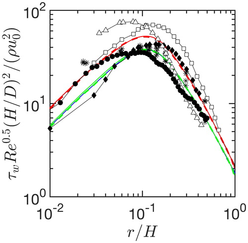
Figure 7. Simulated stagnation pressure p_s, plotted against simulated maximum wall shear stress τ_w,max. Legend: solid black line – linear regression with zero intercept; dashed red line – second order polynomial regression. Coefficient of determination for linear regression with zero intercept: R²_adj = 0.98331.

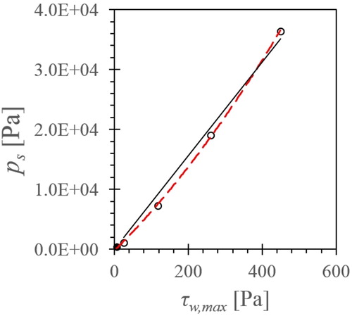
Figure 8. Simulated wall surface forces as a function of ρu₀²/(H/D)²: (a) stagnation pressure p_s, and (b) maximum wall shear stress τ_w,max. Left-hand side: solid black line – linear regression with zero intercept; dashed red line – second order polynomial regression. Right-hand side: residuals correspond to the linear regression with zero intercept. Coefficient of determination for linear regressions with zero intercept: R²_adj (p_s) = 0.99992, R²_adj (τ_w,max) = 0.98323.

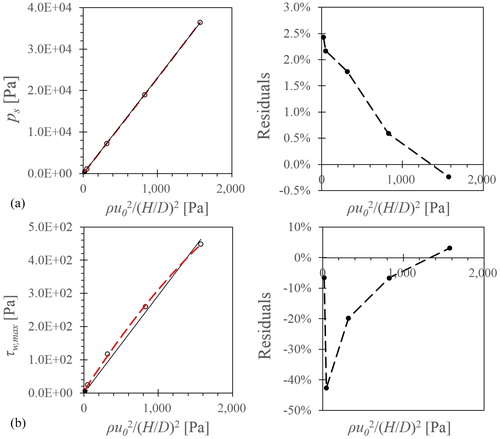
Table 4. Slope, m, and adjusted correlation coefficients, R²_adj, for stagnation pressure p_s and maximum wall shear stress τ_w,max, as functions of different scaling parameters.

Scaling parameter	Slope m (R^2adj), this study		Slope m (R^2adj), reference
	ps	τw,max	ps	τw,max
ρu0^2/(H/D)^2	23.1 (0.99992)	0.294 (0.98323)	27.7 (0.99423)	0.150 (0.95665)
ρu0^2Re^−1/2/(H/D)^2	4,341 (0.95645)	55.7 (0.99265)	7,380 (0.94964)	40.9 (0.96175)
ρu0^2Re^−0.3159/(H/D)^2	634 (0.98326)	8.11 (0.99998)	949 (0.97509)	5.22 (0.96996)

Footnote to Table 4: Reference studies: Bradshaw & Love 1961; Beltaos & Rajaratnam 1974; Hanson, Robinson, and Temple 1990; Shademan, Balachandar, and Barron 2013; Shademan et al. 2016 (please refer to Supplemental material).

Figure 9. Simulated wall surface forces as a function of ρu₀²/Re^−1/2/(H/D)²: (a) stagnation pressure p_s, and (b) maximum wall shear stress τ_w,max. Left-hand side: solid black line – linear regression with zero intercept; dashed red line – second order polynomial regression. Right-hand side: residuals correspond to the linear regression with zero intercept. Coefficient of determination for linear regressions with zero intercept: R²_adj (p_s) = 0.95645, R²_adj (τ_w,max) = 0.99265.

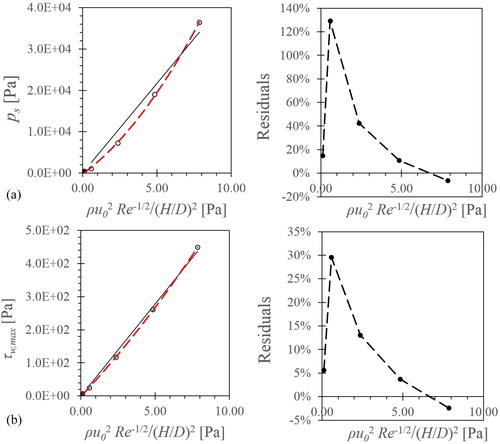
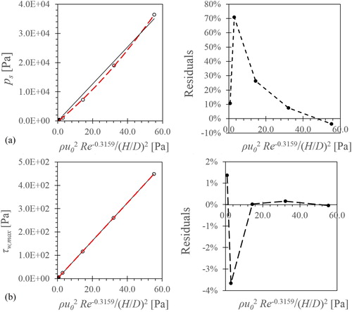
Figure 10. Simulated wall surface forces as a function of ρu₀²/Re^−0.3159/(H/D)²: (a) stagnation pressure p_s, and (b) maximum wall shear stress τ_w,max. Left-hand side: solid black line – linear regression with zero intercept; dashed red line – second order polynomial regression. Right-hand side: residuals correspond to the linear regression with zero intercept. Coefficient of determination for linear regressions with zero intercept: R²_adj (p_s) = 0.98326, R²_adj (τ_w,max) = 0.99998.

Bradshaw P, Love EM. 1961. The normal impingement of a circular air jet on a flat surface. Reports and Memoranda No. 3205. London (UK).

 Google Scholar

Poreh M, Tsuei YG, Cermak JE. 1967. Investigation of a turbulent radial wall jet. J Appl Mech. 34:457–463. doi: 10.1115/1.3607705

 Web of Science ®Google Scholar

Kataoka K, Mizushina T. 1974. Local enhancement of the rate of heat transfer in an impinging round jet by free-stream turbulence. In: Kaigi NG, Kyōkai KK, Gakkai NK, editors. Proc 5th Int Heat Transf Conf. Tokyo (Japan); p. 305–309.

 Google Scholar

Beltaos S, Rajaratnam N. 1974. Impinging circular turbulent jets. ASCE J Hydraul Div. 100:1313–1328.

 Google Scholar

Giralt F, Chia C-J, Trass O. 1977. Characterization of the impingement region in a axisymmetric turbulent jet. Ind Eng Chem Fund. 16:21–28. doi: 10.1021/i160061a007

 Web of Science ®Google Scholar

Hanson GJ, Robinson KM, Temple DM. 1990. Pressure and stress distributions due to a submerged impinging jet. Proceedings of the 1990 National Conference ASCE, Vol. 1. pp. 525–530. San Diego, CA, Jul 30–Aug 3, 1990.

 Google Scholar

Alekseenko SV, Markovich DM. 1994. Electrodiffusion diagnostics of wall shear stresses in impinging jets. J Appl Electrochem. 24:626–631. doi: 10.1007/BF00252087

 Web of Science ®Google Scholar

Phares DJ, Smedley GT, Flagan RC. 2000. The wall shear stress produced by the normal impingement of a jet on a flat surface. J Fluid Mech. 418:351–375. doi: 10.1017/S002211200000121X

 Web of Science ®Google Scholar

Shademan M, Balachandar R, Barron RM. 2013. CFD analysis of the effect of nozzle stand-off distance on turbulent impinging jets. Can J Civ Eng. 40:603–612. doi: 10.1139/cjce-2012-0199

 Web of Science ®Google Scholar

Ghaneeizad SM, Atkinson JF, Bennett SJ. 2015. Effect of flow confinement on the hydrodynamics of circular impinging jets: implications for erosion assessment. Environ Fluid Mech. 15:1–25. doi: 10.1007/s10652-014-9354-3

 Web of Science ®Google Scholar

Shademan M, Balachandar R, Roussinova V, Barron R. 2016. Round impinging jets with relatively large stand-off distance. Phys Fluids. 28:075107. doi: 10.1063/1.4955167

 Web of Science ®Google Scholar

Roache PJ. 1994. Perspective: a method for uniform reporting of grid refinement studies. J Fluids Eng. 116:405–413. doi: 10.1115/1.2910291

 Web of Science ®Google Scholar