Two-dimensional core-softened model with water like properties: solvation of non-polar solute

Figures & data

Figure 1. The solvent–solvent interaction $U\left(r\right)$ (solid line), the LJ contribution (long dashed line) and the Gaussian part (dashed line).

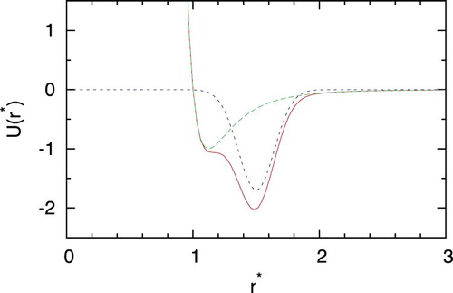
Figure 2. Comparison of the correlation function for different closures with Monte Carlo simulation results for ${\sigma }_{22}$=1.0, temperature $T^{\ast }=1.5$, ${\rho }_1^{\ast }=0.3$, ${\rho }_2^{\ast }=0.1$. Monte Carlo results are plotted with symbols, and IET by lines. Results are for closures (a) SMSA, (b) PY and (c) KH. Red line and symbols are for $g_{11}\left(r^{\ast }\right)$, green for $g_{12}\left(r^{\ast }\right)$ and blue for $g_{22}\left(r^{\ast }\right)$. Different correlation functions are shifted for 1 in y direction. HNC does not converge for this state point.

Figure 3. Comparison of the correlation function for different closures with Monte Carlo simulation results for ${\sigma }_{22}$=1.0, temperature $T^{\ast }=1.5$, ${\rho }_1^{\ast }=0.1$, ${\rho }_2^{\ast }=0.2$. Monte Carlo results are plotted with symbols, and IET by lines. Results are for closures (a) SMSA, (b) PY, (c) KH and (d) HNC. Legend as in Figure 2.

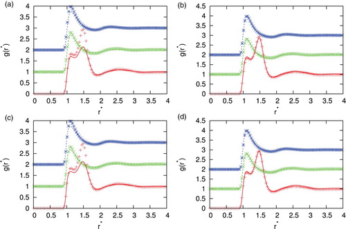
Figure 4. Comparison of the correlation function for different closures with Monte Carlo simulation results for ${\sigma }_{22}$=2.0, temperature $T^{\ast }=1.5$, ${\rho }_1^{\ast }=0.3$, ${\rho }_2^{\ast }=0.05$. Monte Carlo results are plotted with symbols, and IET by lines. Results are for closures (a) SMSA, (b) PY and (c) KH. Legend as in Figure 2. HNC does not converge for this state point.

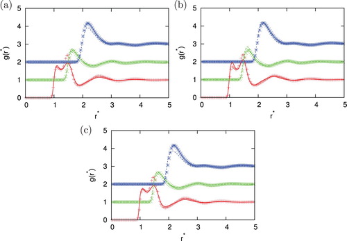
Figure 5. Comparison of the correlation function for different closures with Monte Carlo simulation results for ${\sigma }_{22}$=2.0, temperature $T^{\ast }=1.5$, ${\rho }_1^{\ast }=0.3$, ${\rho }_2^{\ast }=0.15$. Monte Carlo results are plotted with symbols, and IET by lines. Results are for closures (a) SMSA, (b) PY and (c) KH. Legend as in Figure 2. HNC does not converge for this state point.

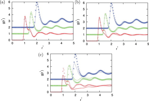
Figure 6. Comparison of the correlation function for different closures with Monte Carlo simulation results for ${\sigma }_{22}$=0.5, temperature $T^{\ast }=1.5$, ${\rho }_1^{\ast }=0.3$, ${\rho }_2^{\ast }=0.1$. Monte Carlo results are plotted with symbols, and IET by lines. Results are for closures (a) SMSA, (b) PY, (c) KH and (d) HNC. Legend as in Figure 2.

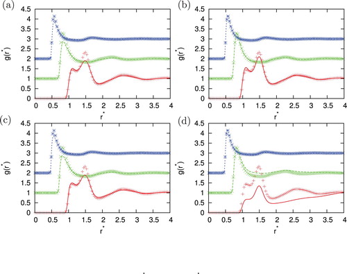
Figure 7. Comparison of the correlation function for different closures with Monte Carlo simulation results for ${\sigma }_{22}$=0.5, temperature $T^{\ast }=1.5$, ${\rho }_1^{\ast }=0.1$, ${\rho }_2^{\ast }=0.2$. Monte Carlo results are plotted with symbols, and IET by lines. Results are for closures (a) SMSA, (b) PY, (c) KH and (d) HNC. Legend as in Figure 2.

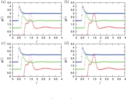
Figure 8. Density dependence of internal energy per particle for ${\sigma }_{22}$=1.00 at (a) $T^{\ast }=2.0$, ${\rho }_2^{\ast }=0.1$ (b) $T^{\ast }=1.5$, ${\rho }_2^{\ast }=0.05$ and (c) $T^{\ast }=1.0$, ${\rho }_2^{\ast }=0.2$. Monte Carlo results are plotted with symbols, SMSA with solid red line, PY with long dashed green line, HNC with dashed blue line and KH with dotted pink line.

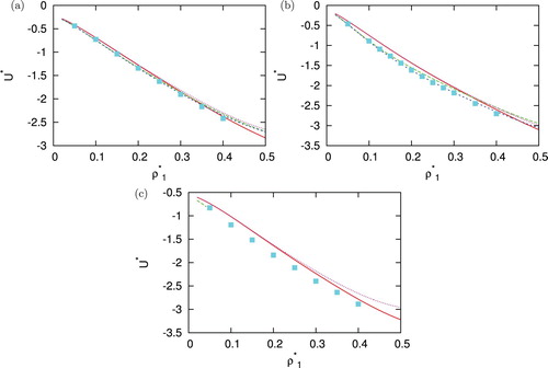
Figure 9. Density dependence of pressure per particle for ${\sigma }_{22}$=1.00 at (a) $T^{\ast }=2.0$, ${\rho }_2^{\ast }=0.1$ (b) $T^{\ast }=1.5$, ${\rho }_2^{\ast }=0.05$ and (c) $T^{\ast }=1.0$, ${\rho }_2^{\ast }=0.2$. Monte Carlo results are plotted with symbols, SMSA with solid red line, PY with long dashed green line, HNC with dashed blue line and KH with dotted pink line.

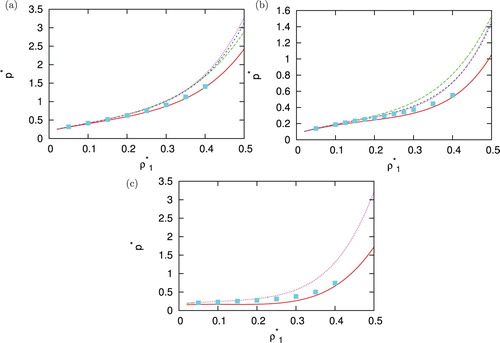
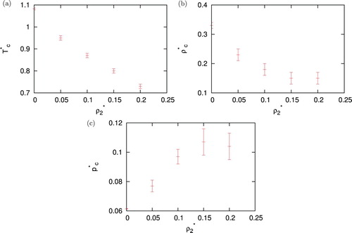
Figure 10. Monte Carlo results for (a) critical temperature, (b) density and (c) pressure as function of ${\rho }_2$ for same size of solute ${\sigma }_{22}$=1.0 as solvent.