RUPTURA: simulation code for breakthrough, ideal adsorption solution theory computations, and fitting of isotherm models

Figures & data

Figure 1. (Colour online) Schematic diagram of fixed-bed adsorber. A peristaltic compressor/pump is used to maintain a constant flow rate. In most gas-phase adsorbers, the gas enters from the top and flows down through the bed, while in a typical liquid system the column fills upwards [18]. The outlet of the bed is connected to a sample collector.

Table 1. Isotherm models, Henry and saturation regime, and the order of input of the arguments in RUPTURA.

Model	Equation	Henry	saturation	$b_0$	$b_1$	$b_2$
Langmuir [46]	$q\left(p\right)=q^{\mathrm{s}\mathrm{a}\mathrm{t}}\frac{bp}{1+bp}$	$b{q}^{\mathrm{s}\mathrm{a}\mathrm{t}}$	$q^{\mathrm{s}\mathrm{a}\mathrm{t}}$	$q^{\mathrm{s}\mathrm{a}\mathrm{t}}$	b
n-site Langmuir	$q\left(p\right)=\sum _i{q}_i^{\mathrm{s}\mathrm{a}\mathrm{t}}\frac{b_{i}p}{1+b_{i}p}$	$\sum _i{b}_i{q}^{\mathrm{s}\mathrm{a}\mathrm{t}}$	$\sum _i{q}_i^{\mathrm{s}\mathrm{a}\mathrm{t}}$	$q^{\mathrm{s}\mathrm{a}\mathrm{t}}$	b
BET [47]	$q\left(p/p^0\right)=q^{\mathrm{s}\mathrm{a}\mathrm{t}}\frac{b\left(p/p^0\right)}{(1-c(p/p^0\left)\right)(1-c+b(p/p^0\left)\right)}$	$\frac{b{q}^{\mathrm{s}\mathrm{a}\mathrm{t}}}{1-c}$	$\frac{b{q}^{\mathrm{s}\mathrm{a}\mathrm{t}}}{(1-c)(1-c+b)}$	$q^{\mathrm{s}\mathrm{a}\mathrm{t}}$	b	c
Anti-Langmuir [24]	$q\left(p\right)=\frac{ap}{1-bp}$	a	✗	a	b
Henry	$q\left(p\right)=ap$	a	✗	a
Freundlich [48]	$q\left(p\right)=a{p}^{1/\nu }$	✗	✗	a	ν
Sips [49]	$q\left(p\right)=q^{\mathrm{s}\mathrm{a}\mathrm{t}}\frac{(bp{)}^{1/\nu }}{1+(bp{)}^{1/\nu }}$	✗	$q^{\mathrm{s}\mathrm{a}\mathrm{t}}$	$q^{\mathrm{s}\mathrm{a}\mathrm{t}}$	b	ν
n-site Sips	$q\left(p\right)=\sum _i{q}_i^{\mathrm{s}\mathrm{a}\mathrm{t}}\frac{(b_{i}p{)}^{1/{\nu }_i}}{1+(b_{i}p{)}^{1/{\nu }_i}}$	✗	$\sum _i{q}_i^{\mathrm{s}\mathrm{a}\mathrm{t}}$	$q^{\mathrm{s}\mathrm{a}\mathrm{t}}$	b	ν
Langmuir-Freundlich [50]	$q\left(p\right)=q^{\mathrm{s}\mathrm{a}\mathrm{t}}\frac{b{p}^{\nu }}{1+b{p}^{\nu }}$	✗	$q^{\mathrm{s}\mathrm{a}\mathrm{t}}$	$q^{\mathrm{s}\mathrm{a}\mathrm{t}}$	b	ν
n-site Langmuir-Freundlich	$q\left(p\right)=\sum _i{q}_i^{\mathrm{s}\mathrm{a}\mathrm{t}}\frac{b_i{p}_i^{\nu }}{1+b_i{p}_i^{\nu }}$	✗	$\sum _i{q}_i^{\mathrm{s}\mathrm{a}\mathrm{t}}$	$q^{\mathrm{s}\mathrm{a}\mathrm{t}}$	b	ν
Redlich-Peterson [51]	$q\left(p\right)=\frac{ap}{1+b{p}^{\nu }}$	a	✗	a	b	ν
Toth [52–54]	$q\left(p\right)=q^{\mathrm{s}\mathrm{a}\mathrm{t}}\frac{bp}{[1+(bp{)}^{\nu }{]}^{1/\nu }}$	$b{q}^{\mathrm{s}\mathrm{a}\mathrm{t}}$	$q^{\mathrm{s}\mathrm{a}\mathrm{t}}$	$q^{\mathrm{s}\mathrm{a}\mathrm{t}}$	b	ν
Unilan	$q\left(p\right)=q^{\mathrm{s}\mathrm{a}\mathrm{t}}\frac{1}{2\eta }\ln \left[\frac{1+b{e}^{\eta }p}{1+b{e}^{-\eta }p}\right]$	$b{q}^{\mathrm{s}\mathrm{a}\mathrm{t}}$	$q^{\mathrm{s}\mathrm{a}\mathrm{t}}$	$q^{\mathrm{s}\mathrm{a}\mathrm{t}}$	b	η
O'Brien & Myers [55]	$q\left(p\right)=q^{\mathrm{s}\mathrm{a}\mathrm{t}}[\frac{bp}{1+bp}+{\sigma }^2\frac{bp(1-bp)}{2(1+bp{)}^3}]$	$q^{\mathrm{s}\mathrm{a}\mathrm{t}}b(1+\frac{{\sigma }^2}{2})$	$q^{\mathrm{s}\mathrm{a}\mathrm{t}}$	$q^{\mathrm{s}\mathrm{a}\mathrm{t}}$	b	σ
Quadratic [56,57]	$q\left(p\right)=q^{\mathrm{s}\mathrm{a}\mathrm{t}}\frac{bp+2c{p}^2}{1+bp+c{p}^2}$	$b{q}^{\mathrm{s}\mathrm{a}\mathrm{t}}$	$2q^{\mathrm{s}\mathrm{a}\mathrm{t}}$	$q^{\mathrm{s}\mathrm{a}\mathrm{t}}$	b	c
Asymptotic Temkin [58,59]	$q\left(p\right)=q^{\mathrm{s}\mathrm{a}\mathrm{t}}\frac{bp}{1+bp}+q^{\mathrm{s}\mathrm{a}\mathrm{t}}\theta {\left(\frac{bp}{1+bp}\right)}^2(\frac{bp}{1+bp}-1)$	$b{q}^{\mathrm{s}\mathrm{a}\mathrm{t}}$	$q^{\mathrm{s}\mathrm{a}\mathrm{t}}$	$q^{\mathrm{s}\mathrm{a}\mathrm{t}}$	b	θ
Bingel & Walton [45]	$q\left(p\right)=q^{\mathrm{s}\mathrm{a}\mathrm{t}}\frac{1-\exp [-(a+b\left)p\right]}{1+\left(b/a\right)\exp [-(a+b\left)p\right]}$	$a{q}^{\mathrm{s}\mathrm{a}\mathrm{t}}$	$q^{\mathrm{s}\mathrm{a}\mathrm{t}}$	$q^{\mathrm{s}\mathrm{a}\mathrm{t}}$	a	b

Table 2. Isotherm models and their inverse.

Model	inverse
Langmuir	$p\left(q\right)=\frac{q}{b(q^{\mathrm{s}\mathrm{a}\mathrm{t}}-q)}$
n-site Langmuir	numerical
BET	$p\left(q\right)=\frac{-b{q}^{\mathrm{s}\mathrm{a}\mathrm{t}}+bq-cq+c^{2}q\pm \sqrt{4bcq(q-cq)+(-b{q}^{\mathrm{s}\mathrm{a}\mathrm{t}}+bq-cq+c^{2}q{)}^2}}{2bcq}$
Anti-Langmuir	$p\left(q\right)=\frac{q}{(a+bq)}$
Henry	$p\left(q\right)=q/a$
Freundlich	$p\left(q\right)={\left(\frac{q}{a}\right)}^{\nu }$
Sips	$p\left(q\right)=\frac{1}{b}{\left(\frac{q}{q^{\mathrm{s}\mathrm{a}\mathrm{t}}-q}\right)}^{\nu }$
n-site Sips	numerical
Langmuir-Freundlich	$p\left(q\right)={\left(\frac{q}{q^{\mathrm{s}\mathrm{a}\mathrm{t}}b-qb}\right)}^{1/\nu }$
n-site Langmuir-Freundlich	numerical
Redlich-Peterson	numerical
Toth	$p\left(q\right)=\frac{q}{(q^{\mathrm{s}\mathrm{a}\mathrm{t}}b-qb){)}^{1/\nu }}$
Unilan	$p\left(q\right)=\frac{e^{\eta }(\exp (\frac{2\eta q}{q^{\mathrm{s}\mathrm{a}\mathrm{t}}})-1)}{b(e^{2\eta }-\exp (\frac{2\eta q}{q^{\mathrm{s}\mathrm{a}\mathrm{t}}}\left)\right)}$
O'Brien & Myers	not shown here
Quadratic	$p\left(q\right)=\frac{-b{q}^{\mathrm{s}\mathrm{a}\mathrm{t}}+bq\pm \sqrt{(b{q}^{\mathrm{s}\mathrm{a}\mathrm{t}}-bq{)}^2+4q(2c{q}^{\mathrm{s}\mathrm{a}\mathrm{t}}-cq)}}{2(2c{q}^{\mathrm{s}\mathrm{a}\mathrm{t}}-cq)}$
Asymptotic Temkin	not shown here
Bingel & Walton [45]	numerical

Notes: The inverse of the O'Brien & Myers and Temkin model are too long to write down here, but can easily be computed symbolically using Mathematica. Note that multi-site combinations will always need to be computed numerically.

Table 3. Reduced grand potential for isotherm models.

Model	reduced grand potential $\psi \left(p\right)$
Langmuir [23]	$\psi \left(p\right)=q^{\mathrm{s}\mathrm{a}\mathrm{t}}\ln [1+bp]$
n-site Langmuir [23]	$\psi \left(p\right)=\sum _i{q}_i^{\mathrm{s}\mathrm{a}\mathrm{t}}\ln [1+b_{i}p]$
BET [63]	$\psi \left(p\right)=q^{\mathrm{s}\mathrm{a}\mathrm{t}}\ln \left[\frac{1+bp-cp}{1-cp}\right]$
Anti-Langmuir [24]	$\psi \left(p\right)=-\frac{a}{b}\ln [1-bp]$
Henry	$\psi \left(p\right)=ap$
Freundlich [23]	$\psi \left(p\right)=a\nu p^{1/\nu }$
Sips [23]	$\psi \left(p\right)=q^{\mathrm{s}\mathrm{a}\mathrm{t}}\nu \ln [1+(bp{)}^{1/\nu }]$
n-site Sips	$\psi \left(p\right)=\sum _i{q}_i^{\mathrm{s}\mathrm{a}\mathrm{t}}\nu \ln [1+(b_{i}p{)}^{1/{\nu }_i}]$
Langmuir-Freundlich [73]	$\psi \left(p\right)=\frac{q^{\mathrm{s}\mathrm{a}\mathrm{t}}}{\nu }\ln [1+b{p}^{\nu }]$
n-site Langmuir-Freundlich	$\psi \left(p\right)=\sum _i\frac{q_i^{\mathrm{s}\mathrm{a}\mathrm{t}}}{{\nu }_i}\ln [1+b_i{p}^{{\nu }_i}]$
Redlich-Peterson [74,75]	$\begin{array}{rl}\psi \left(p\right)& =ap{}_2{F}_1(1,1/\nu ,1+1/\nu ,-b{p}^{\nu })\\ & (b{p}^{\nu }<1)\\ & =\frac{a}{\nu b^{1/\nu }}[\frac{\pi }{\sin \left(\pi /\nu \right)}+{\displaystyle \sum _{k=1}^{\mathrm{\infty }}(-1{)}^k\frac{(\frac{1}{b{p}^{\nu }}{)}^{k-1/\nu }}{k-1/\nu }}]\\ & (b{p}^{\nu }>1)\end{array}$
Toth [73,76]	$\begin{array}{rl}\psi \left(p\right)& =q^{\mathrm{s}\mathrm{a}\mathrm{t}}bq{}_2{F}_1(1/\nu ,1/\nu ,1+1/\nu ,-(pb{)}^{\nu })\\ & (b{p}^{\nu }<1)\\ & =q^{\mathrm{s}\mathrm{a}\mathrm{t}}(\theta -\frac{\theta }{\nu }\ln [1-{\theta }^{\nu }]-{\displaystyle \sum _{k=1}^{\mathrm{\infty }}\frac{{\theta }^{k\nu +1}}{k\nu [k\nu +1]}})\end{array}$
Unilan [73]	$\psi \left(p\right)=q^{\mathrm{s}\mathrm{a}\mathrm{t}}\frac{1}{2\eta }\left({\mathrm{L}\mathrm{i}}_2\right(-b{e}^{-\eta }p)-{\mathrm{L}\mathrm{i}}_2(-b{e}^{\eta }p\left)\right)$
O'Brien & Myers [23,74]	$\psi \left(p\right)=q^{\mathrm{s}\mathrm{a}\mathrm{t}}[\ln [1+bp]+\frac{{\sigma }^{2}bp}{2(1+bp{)}^2}]$
Quadratic [63]	$\psi \left(p\right)=q^{\mathrm{s}\mathrm{a}\mathrm{t}}\ln [1+bp+c{p}^2]$
Asymptotic Temkin [77]	$\psi \left(p\right)=q^{\mathrm{s}\mathrm{a}\mathrm{t}}(\ln [1+bp]-\frac{1}{2}\theta {\left(\frac{bp}{1+bp}\right)}^2)$
Bingel & Walton [45]	numerical

Notes: The potentials are additive for multi-site models. Note that our expression for the Unilan is the same as Santori et al. [73] but several terms in their expression actually cancel out. Note that the expression for Asymptotic Temkin of Simon et al. [77] contains typos. The dilogarithm function $\left({\mathrm{L}\mathrm{i}}_2\right)$ defined by the power series ${\mathrm{L}\mathrm{i}}_2\left(z\right)=\sum _{n=1}^{\mathrm{\infty }}\frac{z^n}{n^2}\left|z\right|<1$. In RUPTURA, we use the freely available implementation by Alexander Voigt [78]. The hypergeometric function ${}_2{F}_1$ defined by the power series for $\left|z\right|<1$ [79] ${}_2{F}_1(a,b;c;z)=\sum _{k=0}^{\mathrm{\infty }}\frac{\left(a{)}_k\right(b{)}_k}{(c{)}_k}\frac{z^k}{k!}$ where $(q{)}_k$ is the (rising) Pochhammer symbol. The hypergeometric function can be computed by e.g. Gosper's algorithm [80]. Note that the computation of the reduced grand potential for Redlich-Peterson and Toth isotherms is hence computationally much more expensive than for the other isotherm models.

Table 4. Sorption pressures for isotherm models.

Model	sorption pressure $p^{\ast }\left(\psi \right)$
Langmuir	$p^{\ast }\left(\psi \right)=\frac{1}{b}(\exp [\psi /q^{\mathrm{s}\mathrm{a}\mathrm{t}}]-1)$
n-site Langmuir	numerical
BET	numerical
Anti-Langmuir	$p^{\ast }\left(\psi \right)=\frac{1}{b}(1-\exp [-\psi b/a])$
Henry	$p^{\ast }\left(\psi \right)=\frac{\psi }{a}$
Freundlich	$p^{\ast }\left(\psi \right)={\left(\frac{\psi }{a\nu }\right)}^{\nu }$
Sips	$p^{\ast }\left(\psi \right)=\frac{1}{b}{(\exp \left[\frac{\psi }{\nu q^{\mathrm{s}\mathrm{a}\mathrm{t}}}\right]-1)}^{\nu }$
n-site Sips	numerical
Langmuir-Freundlich	$p^{\ast }\left(\psi \right)={\left(\frac{\exp \left[\nu \psi /q^{\mathrm{s}\mathrm{a}\mathrm{t}}\right]-1}{b}\right)}^{1/\nu }$
n-site Langmuir-Freundlich	numerical
Redlich-Peterson	numerical
Toth	numerical
Unilan	numerical
O'Brien & Myers	numerical
Quadratic	$p^{\ast }\left(\psi \right)=\frac{-b\pm \sqrt{b^2-4c+3c\exp \left[\psi /q^{\mathrm{s}\mathrm{a}\mathrm{t}}\right]}}{2c}$
Asymptotic Temkin	numerical
Bingel & Walton	numerical

Notes: Models with an analytical inverse for the reduced grand potential are an order of magnitude faster than models that have to be numerically inverted.

Figure 2. (Colour online) IAST algorithm: (a) adsorbed phase mole fraction as a function of the reduced grand potential (b) graphical representation of the basic IAST relationship. The sum of the adsorbed phase mole fractions is unity at reduced grand potential $\psi =13.6755$ mol/(kg framework). By using $\left(\sum _i{x}_i\right)-1$, a root-finding algorithm can be used. Note that that $\sum _i{x}_i$ has a monotonic relation to the reduced grand potential, hence it is also amendable to bi-section methods.

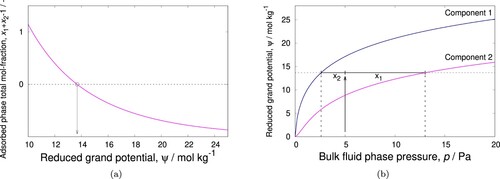
Figure 3. (Colour online) Example of IAST prediction for a binary mixture described by Langmuir-Freundlich isotherms. At 5 Pa total pressure and gas-phase mole fractions $y_1=0.4$ and $y_2=0.6$, we find adsorbed absolute loadings of $q_1=3.92$ and $q_2=1.17$ mol/kg. Typically in a mixture, a component with the highest saturation loading will drive the other components out at high pressures.

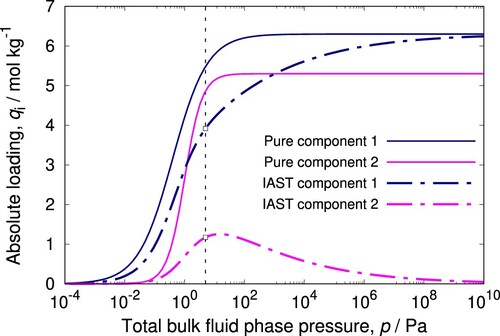
Figure 4. (Colour online) Schematic representation of the Segregated Explicit Isotherm (SEI) model which accounts for the separate thermodynamic equilibrium of the adsorbed phases with the gas phase at different adsorption sites. Each adsorbed phase is separately in thermodynamic equilibrium with the gas phase and it is represented by the adsorption isotherm proposed by Van Assche et al. [30]. The gas phase has a total pressure of $p_{{}_T}$ and the gas phase mole fractions of the components in the mixture are represented by y. In the adsorbed phase j, the loading of the component i is $q_{i,j}$.

Algorithm 1 Procedure for calculating the equilibrium loadings for components in mixtures using the analytic approach of Van Assche et al. [30].

Arrange the components in ascending order based on the value of the saturation loadings $\left(q^{\mathrm{s}\mathrm{a}\mathrm{t}}\right)$.

$q_1^{\mathrm{s}\mathrm{a}\mathrm{t}}\le q_2^{\mathrm{s}\mathrm{a}\mathrm{t}}\cdots \le q_{N_{{}_C}-1}^{\mathrm{s}\mathrm{a}\mathrm{t}}\le q_{N_{{}_C}}^{\mathrm{s}\mathrm{a}\mathrm{t}}$

Calculate the ratios of $q_i^{\mathrm{s}\mathrm{a}\mathrm{t}}$ $\left(n_i\right)$ for each component

$n_i=\frac{q_i^{\mathrm{s}\mathrm{a}\mathrm{t}}}{q_{i-1}^{\mathrm{s}\mathrm{a}\mathrm{t}}}$ $n_1=1$

${\alpha }_i=({\alpha }_{i+1}+k_i{p}_i{)}^{n_i}$

${\alpha }_{N_{{}_C}+1}=1$

Equilibrium loading for each component at the jth site $q_i=q_i^{\mathrm{s}\mathrm{a}\mathrm{t}}{k}_i{p}_i\frac{1}{{\alpha }_1}\prod _{m=1}^i\frac{{\alpha }_{m,}}{{\alpha }_{m+1}+k_m{p}_m}$

Rearrange the adsorbed loadings in the original order as provided in the input.

return $q_i$

Figure 5. (Colour online) Equilibrium of each of the adsorbed phases with the gas phase in the Segregated Ideal Adsorbed Solution Theory (SIAST) model [29]. Each adsorbed phase is separately in equilibrium with the gas phase. The system is at a constant temperature. The gas phase has a total pressure of $p_{\mathrm{t}\mathrm{o}\mathrm{t}}$ and the mole fraction of component i equals $y_i$. In the adsorbed phase j, the loading of component i is $q_{ij}$.

Figure 6. (Colour online) Numerical procedure to calculate equilibrium loadings for a binary mixture developed by Mirzaei et al. [118]. The bulk phase concentrations are the input to this approach and the adsorbed mole fraction for component 1 $\left(x_1\right)$ is used as the guessed value. Based on $x_1$, $x_2$ is estimated. Further, the grand potentials for components 1 and 2 are calculated separately and the difference between these two values are computed. If the difference is less than the predefined error value, then the total equilibrium loadings and the loadings for each component are determined. Otherwise, a new guessed value for component 1 is considered and the steps (3–7) are repeated.

Algorithm 2 IAST calculation using bi-section. The tolerance value ϵ can be set to ${10}^{-15}$.

function IAST(p, $y_i$)
ψ $\leftarrow$ initial value
$\sum _i{x}_i\leftarrow \sum _i{y}_i\times p/p_i^{\ast }\left(\psi \right)$	⊳ /* Equation (47(47) $y_i{p}_{{}_T}=p_i=x_i{p}_i^{\ast }\left(\psi \right)i=1,2,\dots ,N_{{}_C}\left(N_{{}_C}\mathrm{e}\mathrm{q}\mathrm{u}\mathrm{a}\mathrm{t}\mathrm{i}\mathrm{o}\mathrm{n}\mathrm{s}\right)$(47) ) */
${\psi }_{\uparrow }$ $\leftarrow$ ψ	⊳ /* Initialize the top bracket with the inital ψ value */
${\psi }_{\downarrow }$ $\leftarrow$ ψ	⊳ /* Initialize the bottom bracket with the inital ψ value */
if $\sum _i{x}_i>1$ then	⊳ /* bottom bracket known, searching for top bracket */
repeat
${\psi }_{\uparrow }$ $\leftarrow$ 2×${\psi }_{\uparrow }$
$\sum _i{x}_i\leftarrow \sum _i{y}_i\times p/p_i^{\ast }\left({\psi }_{\uparrow }\right)$	⊳ /* Equation (47(47) $y_i{p}_{{}_T}=p_i=x_i{p}_i^{\ast }\left(\psi \right)i=1,2,\dots ,N_{{}_C}\left(N_{{}_C}\mathrm{e}\mathrm{q}\mathrm{u}\mathrm{a}\mathrm{t}\mathrm{i}\mathrm{o}\mathrm{n}\mathrm{s}\right)$(47) ) */
until $\sum _i{x}_i<1$
else	⊳ /* top bracket known, searching for bottom bracket */
repeat
${\psi }_{\downarrow }$ $\leftarrow$ ${\psi }_{\downarrow }/2$
$\sum _i{x}_i\leftarrow \sum _i{y}_i\times p/p_i^{\ast }\left({\psi }_{\downarrow }\right)$	⊳ /* Equation (47(47) $y_i{p}_{{}_T}=p_i=x_i{p}_i^{\ast }\left(\psi \right)i=1,2,\dots ,N_{{}_C}\left(N_{{}_C}\mathrm{e}\mathrm{q}\mathrm{u}\mathrm{a}\mathrm{t}\mathrm{i}\mathrm{o}\mathrm{n}\mathrm{s}\right)$(47) ) */
until $\sum _i{x}_i>1$
end if
repeat
ψ $\leftarrow$ $\frac{1}{2}({\psi }_{\uparrow }+{\psi }_{\downarrow })$	⊳ /* Use bisection to find the ψ within the interval */
$\sum _i{x}_i\leftarrow \sum _i{y}_i\times p/p_i^{\ast }\left(\psi \right)$	⊳ /* Equation (47(47) $y_i{p}_{{}_T}=p_i=x_i{p}_i^{\ast }\left(\psi \right)i=1,2,\dots ,N_{{}_C}\left(N_{{}_C}\mathrm{e}\mathrm{q}\mathrm{u}\mathrm{a}\mathrm{t}\mathrm{i}\mathrm{o}\mathrm{n}\mathrm{s}\right)$(47) ) */
if $\sum _i{x}_i>1$ then	⊳ /* New range is ψ to ${\psi }_{\uparrow }$ */
${\psi }_{\downarrow }$ $\leftarrow$ ψ
else	⊳ /* New range is ${\psi }_{\downarrow }$ to ψ */
${\psi }_{\uparrow }$ $\leftarrow$ ψ
end if
until $\frac{|{\psi }_{\uparrow }-{\psi }_{\downarrow }|}{|{\psi }_{\uparrow }+{\psi }_{\downarrow }|}<ϵ$	⊳ /* Iterate until ${\psi }_{\uparrow }$ and ${\psi }_{\downarrow }$ are equal to within precision ϵ */
ψ $\leftarrow$ $\frac{1}{2}({\psi }_{\uparrow }+{\psi }_{\downarrow })$	⊳ /* Final computed value of the reduced grand potential ψ */
$\sum _i{x}_i\leftarrow \sum _i{y}_i\times p/p_i^{\ast }\left(\psi \right)$	⊳ /* Mole fractions sum to unity (within precision ϵ), Equation (48(48) $\sum _{i=1}^{N_{{}_C}}{x}_i=1\left(1\mathrm{e}\mathrm{q}\mathrm{u}\mathrm{a}\mathrm{t}\mathrm{i}\mathrm{o}\mathrm{n}\right)$(48) ) */
for $i\in \{1,\dots ,N_c\}$ do
$x_i$ $\leftarrow$ $\frac{y_{i}p}{p\left(\psi \right)}$	⊳ /* Equation (47(47) $y_i{p}_{{}_T}=p_i=x_i{p}_i^{\ast }\left(\psi \right)i=1,2,\dots ,N_{{}_C}\left(N_{{}_C}\mathrm{e}\mathrm{q}\mathrm{u}\mathrm{a}\mathrm{t}\mathrm{i}\mathrm{o}\mathrm{n}\mathrm{s}\right)$(47) ) */
end for
$1/q^T$ $\leftarrow$ $\sum _i\frac{x_i}{f\left(p\right(\psi \left)\right)}$	⊳ /* Equation (50(50) $\frac{1}{q_{{}_T}}=\sum _{i=1}^{N_{{}_C}}\frac{x_i}{q_i^{\ast }}$(50) ) */
for $i\in \{1,\dots ,N_c\}$ do
$q_i$ $\leftarrow$ $x_i{q}^T$	⊳ /* Equation (52(52) $q_i=x_i{q}_{{}_T}$(52) ) */
end for
return ψ, $x_i$, $q_i$
end function

Algorithm 3 Inverse computation using bi-section. The tolerance value ϵ can be set to 10^–15.

function $p\left(\psi \right)$

p $\leftarrow$ initial value

$p_{\uparrow }$ $\leftarrow$ p ⊳ /* Initialize the top bracket with the inital p value */

$p_{\downarrow }$ $\leftarrow$ p ⊳ /* Initialize the bottom bracket with the inital p value */ if $\psi \left(\right(p)>1$ then ⊳ /* bottom bracket known, searching for top bracket */  repeat

$p_{\uparrow }$ $\leftarrow$ 2× $p_{\uparrow }$

until $\psi \left(p_{\uparrow }\right)<1$

else ⊳ /* top bracket known, searching for bottom bracket */

repeat

$p_{\downarrow }$ $\leftarrow$ $p_{\downarrow }/2$

until $\psi \left(p_{\downarrow }\right)>1$

end if

repeat

p $\leftarrow$ $\frac{1}{2}(p_{\uparrow }+p_{\downarrow })$ ⊳ /* Use bisection to find the p within the interval */

if $\psi \left(p\right)>1$ then ⊳ /* New range is p to $p_{\uparrow }$ */

$p_{\downarrow }$ $\leftarrow$ p

else ⊳ /* New range is $p_{\downarrow }$ to p */

$p_{\uparrow }$ $\leftarrow$ p

end if

until $\frac{|p_{\uparrow }-p_{\downarrow }|}{|p_{\uparrow }+p_{\downarrow }|}<ϵ$ ⊳ /* Iterate until $p_{\uparrow }$ and $p_{\downarrow }$ are equal to within precision ϵ */

p $\leftarrow$ $\frac{1}{2}(p_{\uparrow }+p_{\downarrow })$

return p

end function

Table 5. Parameters for the O'Brien and Myers adsorption isotherm model considered by Moon and Tien [110] for a 10-component mixture at 300 kPa, $q_{{}_T}=2.3050$ mol/kg and $\sum _i{x}_i=0.9912$.

component	$q_i^{\mathrm{s}\mathrm{a}\mathrm{t}}$ [mol/kg]	$b_i$ [Pa${}^{-1}$]	${\sigma }_i$ [−]	$p_i$ [kPa]	$y_i$ [−]	${\psi }_i$ [mol/kg] (Ref. [110])	${\psi }_i$ [mol/kg] (this work)	$x_i$ [−] (Ref. [110])	$x_i$ [−] (this work)
1	5.0	$1.0\times {10}^{-5}$	1.2	30.0	0.1	4.261	4.19182774500228	0.3129	0.321867
2	3.0	$0.6\times {10}^{-5}$	1.1	30.0	0.1	4.191	4.19182774500229	0.0698	0.069755
3	4.0	$0.09\times {10}^{-5}$	0.8	30.0	0.1	4.194	4.19182774500228	0.0164	0.016412
4	2.0	$1.0\times {10}^{-5}$	1.2	60.0	0.2	4.191	4.19182774500229	0.0926	0.092559
5	3.5	$0.3\times {10}^{-5}$	1.0	30.0	0.1	4.191	4.19182774500228	0.0459	0.045873
6	4.0	$0.1\times {10}^{-5}$	1.1	15.0	0.05	4.201	4.19182774500229	0.0102	0.010241
7	2.0	$1.5\times {10}^{-5}$	1.2	15.0	0.05	4.192	4.19182774500228	0.0347	0.034710
8	2.5	$0.1\times {10}^{-5}$	1.15	15.0	0.05	4.170	4.19182774500228	0.0040	0.003953
9	4.0	$0.01\times {10}^{-5}$	1.0	15.0	0.05	4.145	4.19182774500228	0.0010	0.000980
10	5.5	$0.6\times {10}^{-5}$	1.0	60.0	0.2	4.192	4.19182774500228	0.4037	0.403652

Notes: The tolerance for the results of Moon et al. was ${10}^{-5}$. This work uses a relative precision of ${10}^{-15}$. Our computed total loading is $q_{{}_T}=2.26563527$ mol/kg, and the sum of the adsorbed phase mole fractions $\sum _i{x}_i=1$ is normalised to machine precision.

Table 6. Parameters for the O'Brien and Myers adsorption isotherm model considered by Landau et al. [74] for a 10-component mixture, $q_{{}_T}=2.1142$ mol/kg.

component	$q_i^{\mathrm{s}\mathrm{a}\mathrm{t}}$ [mol/kg]	$b_i$ [Pa${}^{-1}$]	${\sigma }_i$ [−]	$p_i$ [kPa]	$y_i$ [−]	${\psi }_i$ [mol/kg] (Ref. [110])	${\psi }_i$ [mol/kg] (this work)	$q_i$ [mol/kg] (Ref. [74])	$q_i$ [mol/kg] (this work)
1	5.0	$1.0\times {10}^{-5}$	1.2	30.0	0.1	3.68342	3.683573349491790	0.8443	0.845631
2	3.0	$0.6\times {10}^{-5}$	1.1	3.0	0.01	3.68238	3.683573349491790	0.0192	0.019219
3	4.0	$0.09\times {10}^{-5}$	0.8	3.0	0.01	3.69288	3.683573349491789	0.0043	0.004325
4	2.0	$1.0\times {10}^{-5}$	1.2	15.0	0.05	3.68419	3.683573349491789	0.0677	0.067839
5	3.5	$0.3\times {10}^{-5}$	1.0	60.0	0.2	3.68371	3.683573349491791	0.2467	0.247123
6	4.0	$0.1\times {10}^{-5}$	1.1	60.0	0.2	3.68317	3.683573349491790	0.1093	0.109459
7	2.0	$1.5\times {10}^{-5}$	1.2	30.0	0.1	3.68345	3.683573349491791	0.2032	0.203517
8	2.5	$0.1\times {10}^{-5}$	1.15	60.0	0.2	3.68459	3.683573349491790	0.0446	0.044700
9	4.0	$0.01\times {10}^{-5}$	1.0	6.0	0.02	3.76951	3.683573349491788	0.0010	0.001042
10	5.5	$0.6\times {10}^{-5}$	1.0	33.0	0.11	3.68348	3.683573349491788	0.5739	0.574822

Notes: The relative and absolute tolerances for the results of Landau et al. are ${10}^{-10}$ and ${10}^{-12}$, respectively. This work uses a relative precision of ${10}^{-15}$. Our computed total loading is $q_{{}_T}=2.117678$ mol/kg.

Figure 7. (Colour online) Schematic representation of a packed bed adsorber. The packed bed adsorber is a cylindrical column filled with nanoporous adsorbent material (crystalline or amorphous). When a fluid mixture is fed as input to the column, adsorption of various components present in the mixture takes place inside these nanoporous materials.

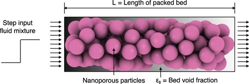
Figure 8. (Colour online) Different zones in a breakthrough curve at the exit of the fixed bed column. Fluid phase concentration of an adsorbing component as a function of time at the fixed bed column outlet. The profile is divided into three zones: (a) the unsaturated zone: where the maximum adsorption takes place, (b) mass transfer zone: where adsorption process progresses rapidly towards equilibrium, (c) saturated zone: where no more adsorption takes place as equilibrium between the fluid and the adsorbed phase is achieved.

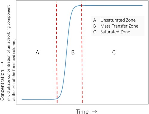
Table 7. Correlations for estimation of axial dispersion coefficient, ${\mathcal{D}}_z$ in fixed bed adsorbers.

Dispersion Model	Conditions	Authors
${\mathcal{D}}_z=\frac{2r_{{}_P}v{ϵ}_{{}_B}}{0.2+0.011{\mathrm{R}\mathrm{e}}^{0.48}}$	${10}^{-3}<\mathrm{R}\mathrm{e}<{10}^3$	Chung and Wen [157]
${\mathcal{D}}_z=0.7D_m+\frac{5r_{{}_P}v}{1+4.4D_m/\left(r_{{}_P}v\right)}$	valid for liquids	De Ligny [156]
${\mathcal{D}}_z=0.7D_m+\frac{2r_{{}_P}v{ϵ}_{{}_B}}{0.18+0.008{\mathrm{R}\mathrm{e}}^{0.59}/\left(r_{{}_P}v\right)}$	–	Rastegar and Gu [158]
${\mathcal{D}}_z=0.73D_m+\frac{0.5d_{\mathrm{p}}v{ϵ}_{{}_B}}{1+\left(9.7D_m\right)/\left(v{ϵ}_{{}_B}{d}_{{}_P}\right)}$	$0.008<\mathrm{R}\mathrm{e}<50,0.0377<d_p<0.60\mathrm{c}\mathrm{m}$	Edwards and Richardson [159]
${\mathcal{D}}_z=\frac{20D_m}{{ϵ}_{{}_B}}+\frac{0.5D_{m}ScRe}{{ϵ}_{{}_B}}$	–	Shafeeyan, da Silva [137,160]
${\mathcal{D}}_z=(0.45+0.55{ϵ}_{{}_B})D_m+r_{{}_P}v$	–	Ruthven [6]

Notes: $D_m$ is the molecular diffusivity, Sc is the Schmidt number and Re is the Reynolds number. $r_{{}_P}$ and $d_{{}_P}$ are the particle radius and particle diameter respectively. v represents velocity and ${ϵ}_{{}_B}$ is the bed porosity.

Figure 9. (Colour online) Loading and concentration profiles according to the pore diffusion model with external mass transfer resistance. The external mass transfer resistance is modeled using the film flux ${\dot{n}}_F\left(t\right)=K_{{}_F}\left(c\right(t)-c_{{}_S}(t\left)\right)$, which is the linear difference of the concentration $c\left(t\right)$ in the bulk solution, and the concentration $c_s\left(t\right)$ at the surface of the crystallite. The flux ${\dot{n}}_T={\dot{n}}_{{}_P}+{\dot{n}}_{{}_S}$ is the sum of the pore diffusion and surface diffusion: ${\dot{n}}_T=D_{{}_P}\mathrm{\partial }{c}_p/\mathrm{\partial }r+{\rho }_{{}_P}{D}_{{}_S}\mathrm{\partial }q/\mathrm{\partial }r$. The continuity of the materials fluxes requires ${\dot{n}}_F={\dot{n}}_{{}_T}$. The surface is considered to be in equilibrium and the adsorbent loading $q(r_p,t)=q\left(p\right(t\left)\right)$ is calculated from the isotherm with functional form q, where the pressure p is related to the surface concentration $c_{{}_S}$ via the ideal gas law as $p=RT{c}_{{}_S}$.

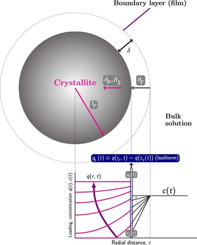
Figure 10. (Colour online) Loading and concentration profiles according to the Linear Driving Force (LDF) model with external mass transfer resistance. The LDF model assumes that there is linear gradient within the solution-side film and within a comparable fictive solid film. The film flux ${\dot{n}}_F\left(t\right)=K_{{}_F}\left(c\right(t)-c_{{}_S}(t\left)\right)$ is the linear difference of the concentration $c\left(t\right)$ in the bulk solution, and the concentration $c_{{}_S}\left(t\right)$ at the surface of the crystallite. The solid flux ${\dot{n}}_{{}_S}$ is the linear difference between the equilibrium loading $q_{{}_S}$ at the surface and the average loading $\overline{q}$: ${\dot{n}}_{{}_S}\left(t\right)={\rho }_{{}_P}{k}_{{}_S}\left(q_{{}_S}\right(t)-\overline{q}(t\left)\right)$, where ${\rho }_{{}_P}$ is the particle density, $k_{{}_S}$ is the intra-particle mass transfer coefficient. The continuity of the materials fluxes requires ${\dot{n}}_{{}_F}={\dot{n}}_{{}_S}$. The surface is considered to be in equilibrium and the adsorbent loading $q(r_{{}_P},t)=q\left(p\right(t\left)\right)$ is calculated from the isotherm with functional form q, where the pressure p is related to the surface concentration $c_{{}_S}$ via the ideal gas law as $p=RT{c}_{{}_S}$.

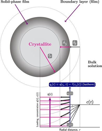
Table 8. First and second order derivatives disretised using the Finite Difference Method (FDM) method [216].

Derivatives	Discretisation	Scheme
$(\frac{\mathrm{\partial }u}{\mathrm{\partial }z}{)}_j$	$\frac{u(j+1)-u\left(j\right)}{\mathrm{\Delta }z}+O\left(\mathrm{\Delta }z\right)$	Forward difference
$(\frac{\mathrm{\partial }u}{\mathrm{\partial }z}{)}_j$	$\frac{u\left(j\right)-u(j-1)}{\mathrm{\Delta }z}+O\left(\mathrm{\Delta }z\right)$	Backward difference
$(\frac{\mathrm{\partial }u}{\mathrm{\partial }z}{)}_j$	$\frac{u(j+1)-u(j-1)}{2\mathrm{\Delta }z}+O(\mathrm{\Delta }z{)}^2$	Central difference
$(\frac{{\mathrm{\partial }}^{2}u}{\mathrm{\partial }{z}^2}{)}_j$	$\frac{u(j+1)-2u\left(j\right)+u(j-1)}{(\mathrm{\Delta }z{)}^2}+O(\mathrm{\Delta }z{)}^2$	Central difference

Figure 11. (Colour online) Algorithm to calculate the breakthrough curve. It is based on the method of lines (MOL) technique to solve the system of differential algebraic equations. Time integration is done using an explicit method called Strong Stability preserving Runge-Kutta (SSP-RK(3,3)) as shown in Equations (292(292) $Y{(t+\mathrm{\Delta }t)}^{\left(1\right)}=Y\left(t\right)+\mathrm{\Delta }tF\left(Y\left(t\right)\right)$(292) )–(294(294) $Y(t+\mathrm{\Delta }t)=\frac{1}{3}Y\left(t\right)+\frac{2}{3}Y{(t+\mathrm{\Delta }t)}^{\left(2\right)}+\frac{2}{3}\mathrm{\Delta }tF\left(Y{(t+\mathrm{\Delta }t)}^{\left(2\right)}\right)$(294) ). We first calculate the temporal derivatives of the partial pressures $\left(p_i\right)$ and the adsorbed loadings $\left({\overline{q}}_i\right)$. Until the final time step is reached, we update the values of $p_i$, $p_{{}_T}$, ${\overline{q}}_i$, $q_{\mathrm{e}\mathrm{q},i}$ and v at each time step.

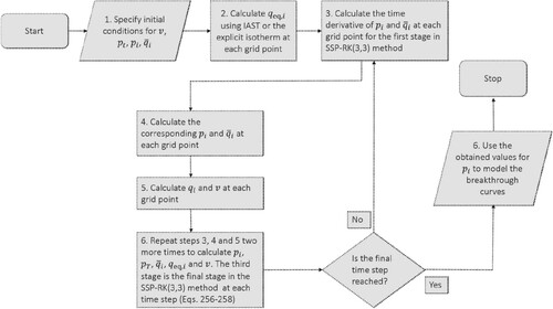
Figure 12. (Colour online) Examples of pulse-style breakthrough curve simulation for the mixture of ${\mathrm{C}}_6$ isomers: n-hexane $\left({\mathrm{n}\mathrm{C}}_6\right)$, 3-methyl pentane $\left(3{\mathrm{m}\mathrm{C}}_5\right)$, 2,2-dimethyl butane $\left(22{\mathrm{d}\mathrm{m}\mathrm{C}}_4\right)$, and 2,3-dimethyl butane $\left(23{\mathrm{d}\mathrm{m}\mathrm{C}}_4\right)$ in BEA-type zeolite at 523 K and 12 bar. Isothermal and isobaric conditions are imposed on the fixed bed column of length (a) 0.1 m and (b) 0.5 m. The bed porosity $\left({ϵ}_{{}_B}\right)$ is 0.2. Helium is used as the carrier gas. The inlet mole fractions for the ${\mathrm{C}}_6$ isomers are considered to be 0.01975. The interstitial velocity (v) at the inlet is 0.019 ms${}^{-1}$. 5s is the pulse time $\left(t_{\mathrm{p}\mathrm{u}\mathrm{l}\mathrm{s}\mathrm{e}}\right)$.

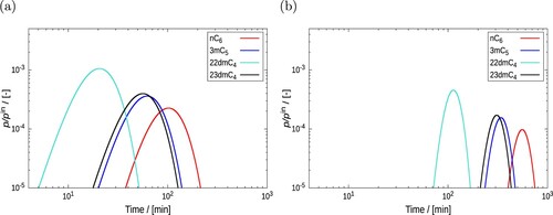
Table 9. Experimental conditions for separation of $2{\mathrm{m}\mathrm{C}}_4$, $2{\mathrm{m}\mathrm{C}}_5$.

	$c_i^{\mathrm{i}\mathrm{n}}/$ [mol m${}^{-3}$]	$p_i^{\mathrm{i}\mathrm{n}}/$ [bar]	$y_i^{\mathrm{i}\mathrm{n}}$
$2{\mathrm{m}\mathrm{C}}_4$	6.27	0.245	0.049
$2{\mathrm{m}\mathrm{C}}_5$	6.60	0.260	0.052

Notes: It includes the inlet concentrations $\left(c_i^{\mathrm{i}\mathrm{n}}\right)$, corresponding partial pressures $\left(p_i^{\mathrm{i}\mathrm{n}}\right)$ and the mole fractions $\left(y_i^{\mathrm{i}\mathrm{n}}\right)$.

Table 10. Values of dispersion coefficient $\left(\mathcal{D}\right)$ and mass transfer coefficient (k) for $2{\mathrm{m}\mathrm{C}}_4$ and $2{\mathrm{m}\mathrm{C}}_5$.

	$\mathcal{D}/$ [m${}^2$ s${}^{-1}$]	$k/$ [s${}^{-1}$]
$2{\mathrm{m}\mathrm{C}}_4$	$4.79\cdot {10}^{-5}$	0.056
$2{\mathrm{m}\mathrm{C}}_5$	$3.91\cdot {10}^{-5}$	0.051

Notes: The coefficients are calculated at 473 K and 5bar for the composition shown in Table 9.

Table 11. Pure component adsorption isotherm parameters.

	$q^{\mathrm{s}\mathrm{a}\mathrm{t}}/$ [mol/(kg framework)]	$b/$ [Pa${}^{-1}$]
$2{\mathrm{m}\mathrm{C}}_4$	$0.717\pm 4\cdot {10}^{-3}$	$2.835\cdot {10}^{-5}\pm 7\cdot {10}^{-7}$
$2{\mathrm{m}\mathrm{C}}_5$	$0.699\pm 2\cdot {10}^{-3}$	$1.271\cdot {10}^{-4}\pm 3\cdot {10}^{-7}$

Notes: Single-site Langmuir isotherms are used to fit the pure component adsorption loading data obtained using GCMC simulations at 473 K. $q^{\mathrm{s}\mathrm{a}\mathrm{t}}$ is the saturation loading and b is the equilibrium constant.

Figure 13. (Colour online) Validation of the breakthrough curve model with the experimental results of Jolimaitre et al. [233]. This figure shows the separation of ${2\mathrm{m}\mathrm{C}}_4$ and ${2\mathrm{m}\mathrm{C}}_5$ in MFI-type zeolite at 473K and 5bar. The coloured squares represent the experimental data and the solid lines represent the results from our simulations.

Figure 14. (Colour online) Adsorption isotherms for CO${}_2$ and C${}_3$H${}_8$ in MOR-type zeolite at 300 K. (a) Unary isotherms (dual-site Langmuir) which are fitted to the pure component loading data obtained using RASPA, (b) comparison between mixture isotherms for equimolar composition of CO${}_2$ and C${}_3$H${}_8$ computed using IAST, SIAST and SEI.

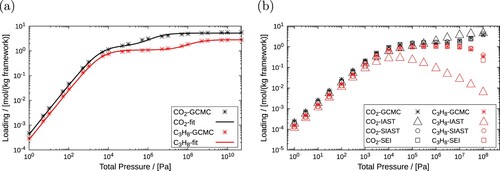
Table 12. Fitted parameters for the adsorption of pure ${\mathrm{C}\mathrm{O}}_2$ and ${\mathrm{C}}_3$ in MOR-type zeolite at 300 K.

	$b_1$	$q_1^{\mathrm{s}\mathrm{a}\mathrm{t}}$	$b_2$	$q_2^{\mathrm{s}\mathrm{a}\mathrm{t}}$
	$\left[1/\mathrm{P}\mathrm{a}\right]$	$\left[\mathrm{m}\mathrm{o}\mathrm{l}/\left(\mathrm{k}\mathrm{g}\mathrm{f}\mathrm{r}\mathrm{a}\mathrm{m}\mathrm{e}\mathrm{w}\mathrm{o}\mathrm{r}\mathrm{k}\right)\right]$	$\left[1/\mathrm{P}\mathrm{a}\right]$	$\left[\mathrm{m}\mathrm{o}\mathrm{l}/\left(\mathrm{k}\mathrm{g}\mathrm{f}\mathrm{r}\mathrm{a}\mathrm{m}\mathrm{e}\mathrm{w}\mathrm{o}\mathrm{r}\mathrm{k}\right)\right]$
${\mathrm{C}\mathrm{O}}_2$	$2.617\cdot {10}^{-4}$	1.60	$4.859\cdot {10}^{-7}$	3.62
	$\pm 3\cdot {10}^{-5}$	$\pm 5\cdot {10}^{-2}$	$\pm 3\cdot {10}^{-8}$	$\pm 5\cdot {10}^{-2}$
${\mathrm{C}}_3$	$6.506\cdot {10}^{-9}$	1.73	$2.376\cdot {10}^{-4}$	1.09
	$\pm 3\cdot {10}^{-10}$	$\pm 6\cdot {10}^{-3}$	$\pm 8\cdot {10}^{-6}$	$\pm 4\cdot {10}^{-3}$

Notes: Adsorbed loadings obtained from the GCMC simulations for the pressure range $({10}^0-5\cdot {10}^{10})$ Pa are fitted using the dual-site Langmuir isotherm.

Table 13. Fitted parameters for the adsorption isotherm (dual-site Langmuir-Freundlich) of o-xylene in MAF-x8-P1 zeolite at 433 K using different methods.

	$q_1^{\mathrm{s}\mathrm{a}\mathrm{t}}/$	$b_1/$	${\nu }_1/$	$q_2^{\mathrm{s}\mathrm{a}\mathrm{t}}/$	$b_2/$	${\nu }_2/$	RMSE/
	[mol/(kg framework)]	[Pa${}^{-1}$]	[–]	[mol/(kg framework)]	[Pa${}^{-1}$]	[–]	[mol/(kg framework)]
RUPTURA	1.9377	1.1132	0.2476	1.5793	$1.0485\times {10}^8$	1.2963	0.062
SciPy	1.9583	1.1334	0.2439	1.5617	$2.8218\times {10}^8$	1.3654	0.062
Gnuplot	1.9554	1.1305	0.2438	1.5642	$2.4394\times {10}^8$	1.3553	0.064
GAIAST	2.0059	1.1785	0.2337	1.5215	$3.2212\times {10}^9$	1.5360	0.066

Notes: In this table, unlike in Figure 20, the Gnuplot fit has been performed using initial values close to the final solution, to avoid being stuck in a local minimum.

Figure 15. (Colour online) Comparison between breakthrough curves obtained on implementing IAST, SIAST, and SEI to the breakthrough curve model. A mixture of CO${}_2$ and C${}_3$H${}_8$ in MOR-type zeolite at 300 K and 10${}^5$ Pa is considered. Each of these components constitutes 10% of the gas phase. Helium is used as the carrier gas. The adsorption column is operated in isothermal and isobaric conditions.

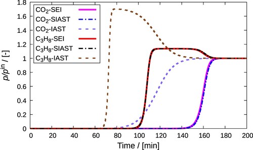
Figure 16. (Colour online) Grid independence test on simulation of breakthrough curves for a mixture of CO${}_2$ and C${}_3$H${}_8$ in MOR-type zeolite at 300 K and 10${}^5$ Pa is performed. (a) Breakthrough curves simulated at different spatial grid points ($N_{\mathrm{g}\mathrm{r}\mathrm{i}\mathrm{d}}=20,50,\mathrm{a}\mathrm{n}\mathrm{d}100$), (b) certain zoomed in parts of the curves showing discrepancies due to the use of a different number of grid points. Each of these components constitutes 10% of the gas phase. Helium is used as the carrier gas. The adsorption column is operated in isothermal and isobaric conditions. With increasing the number of grid points, the breakthrough curves slightly changes. The variation becomes smaller between $N_{\mathrm{g}\mathrm{r}\mathrm{i}\mathrm{d}}=50\mathrm{a}\mathrm{n}\mathrm{d}100$.

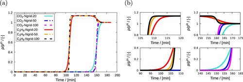
Figure 17. (Colour online) Schematic representation of GA operators crossover, and mutation. The crossover operator is analogous to the crossover that happens during sexual reproduction in biology, and it combines the genotype of two parents to generate new offspring. We implemented three types of crossover operator: with one- and two points, and the uniform crossover. The mutation operator is activated before the children are added to the next generation.

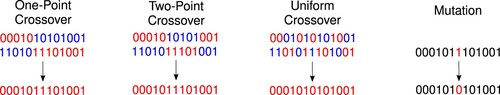
Figure 18. (Colour online) Flowchart of one step, k, in the Nelder-Mead algorithm [117] for a parametric function, f, with two parameters. In this way, the simplex is a triangle, and the visualisation is easier. The four operations and the sorting stage are in green labels.

Figure 19. (Colour online) (Left) Adsorption of n-C${}_7$ in BEA zeolite at 552 K and some fitted models using ISOFIT, Gnuplot, IAST++, and RUPTURA for a Toth model of a single adsorption site. (Right) Predicted loading vale vs. observed loading values. The goodness-of-fit in colours (same code colour of the Left panel) for each code. The RMSE values are in [mol/(kg framework)] units.

Figure 20. (Colour online) (Left) Adsorption of o-xylene in MAF-X8 zeolite at 300 K and some fitted models using IAST++, Gnuplot (from scratch), GAIAST, and RUPTURA for a dual-site Langmuir-Freundlich model. (Right) Predicted loading vale vs. observed loading values. The goodness-of-fit for each code in colours defined in the left panel. The RMSE values are in [mol/(kg framework)] units.

Figure 21. (Colour online) The adsorption isotherm prediction for two, three, and four sites Langmuir-Freundlich isotherm models for o-xylene in MAF-X8. Without the experimental error information for the loading data is difficult to establish what kind of model is more realistic.

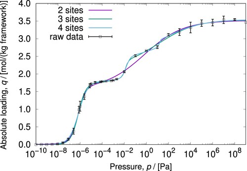
Figure 22. (Colour online) The C${}_6$-alkane-isomers adsorption isotherms in MAF-6 computed from grand-canonical Monte Carlo simulations fitted with dual- and triple site Langmuir-Freundlich isotherm models. The peculiar shape of these isotherms in the low-pressure region makes this system challenging to preform reliable fitting.

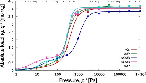
Figure 23. (Colour online) Breakthrough predictions of an equimolar mixture of CO${}_2$-N${}_2$ in silicalite at 313 K and $2.5\cdot {10}^6$ Pa: (a) breakthrough curve plot (file breakthrough_dimensionless.pdf) (b) movie frame of the loading inside the column (file column_movie_Q.mp4).

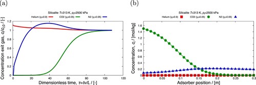
Figure 24. (Colour online) Mixture predictions of a ${\mathrm{C}}_6$ isomer mixture in BEA- type zeolite at 552K using explicit isotherm model developed by Van Assche et al [30]: (a) pure components (file $\mathtt{p}\mathtt{u}\mathtt{r}\mathtt{e}\mathtt{\_}\mathtt{c}\mathtt{o}\mathtt{m}\mathtt{p}\mathtt{o}\mathtt{n}\mathtt{e}\mathtt{n}\mathtt{t}\mathtt{\_}\mathtt{i}\mathtt{s}\mathtt{o}\mathtt{t}\mathtt{h}\mathtt{e}\mathtt{r}\mathtt{m}\mathtt{s}\mathtt{.}\mathtt{p}\mathtt{d}\mathtt{f}$), (b) mixture prediction (file $\mathtt{m}\mathtt{i}\mathtt{x}\mathtt{t}\mathtt{u}\mathtt{r}\mathtt{e}\mathtt{\_}\mathtt{p}\mathtt{r}\mathtt{e}\mathtt{d}\mathtt{i}\mathtt{c}\mathtt{t}\mathtt{i}\mathtt{o}\mathtt{n}\mathtt{.}\mathtt{p}\mathtt{d}\mathtt{f}$).

Figure 25. (Colour online) Fitting a dual site Langmuir isotherm model to the pure component isotherm data for the adsorption of p-xylene in MAF-X8- type zeolite at 433 K. The pure component adsorbed loadings are computed using grand-canonical Monte Carlo simulations. The fitting is performed using genetic algorithm optimisation which is shown in the file $\mathtt{i}\mathtt{s}\mathtt{o}\mathtt{t}\mathtt{h}\mathtt{e}\mathtt{r}\mathtt{m}\mathtt{s}\mathtt{\_}\mathtt{f}\mathtt{i}\mathtt{t}\mathtt{\_}\mathtt{p}\mathtt{-}\mathtt{x}\mathtt{y}\mathtt{l}\mathtt{e}\mathtt{n}\mathtt{e}\mathtt{.}\mathtt{p}\mathtt{d}\mathtt{f}$.

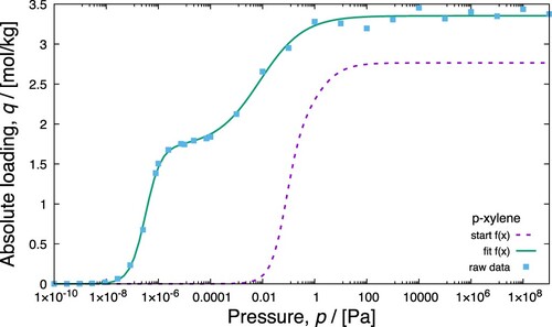
Table 14. List of mixture prediction, breakthrough, and fitting examples provided with RUPTURA.

structure	mixture	$N_{{}_C}$	$N_{\mathrm{g}\mathrm{r}\mathrm{i}\mathrm{d}}$	$\mathrm{\Delta }t$ [s]	$p_i$ [kPa]	$\tau =tv/L$ [−]	time	$p_i$ [kPa]	$\tau =tv/L$ [−]	time
MOR	CO${}_2$-C${}_3$H${}_8$	2	100	0.0005	125.0	270.8	1m36	1250.0	53.2	0m25
JUC-77	xylenes	4	100	0.0005	25.0	201.8	4m02	250.0	43.5	0m58
MIL-125-NH2	xylenes	4	100	0.0005	25.0	355.5	7m34	250.0	77.2	2m07
CoBDP	xylenes	4	100	0.0005	25.0	395.3	8m08	250.0	68.5	1m50
MFI	xylenes	4	100	0.0005	25.0	1025.2	10m13	250.0	162.5	2m08
MIL-47	xylenes	4	100	0.0005	25.0	504.5	11m18	250.0	95.0	2m37
MAF-X8	xylenes	4	100	0.0005	25.0	643.2	13m28	250.0	99.0	2m37
CoBDP	alkanes-C${}_6$	5	100	0.0005	20.0	489.3	13m33	200.0	86.2	2m51
BEA	alkanes-C${}_7$	5	100	0.0005	1.2	873.24	17m10	12.0	331.7	6m57
fe2bdp3	alkanes-C${}_6$	5	100	0.0005	20.0	3520.0	105m58	200.0	376.7	12m41
ZIF-77	alkanes-C${}_5$-C${}_6$-C${}_7$	15	100	0.0005	20.0	269.3	28m03	200.0	52.8	5m44

Notes: For breakthrough simulations, in addition to the $N_{{}_C}$-components, there is a carrier-gas component present. The timings are done on a mac-studio using an M1-chip.

Al Mohammed M, Danish M, Khan I, et al. Continuous fixed bed CO 2 adsorption: breakthrough, column efficiency, mass transfer zone. Processes. 2020;8:1233.

 Web of Science ®Google Scholar

Langmuir I. The adsorption of gases on plane surfaces of glass, mica and platinum. J Am Chem Soc. 1918;40:1361–1403.

 Web of Science ®Google Scholar

Gritti F, Guiochon G. New thermodynamically consistent competitive adsorption isotherm in RPLC. J Colloid Interface Sci. 2003;1:43–59.

 Google Scholar

Guiochon G, Felinger A, Shirazi D. Fundamentals of preparative and nonlinear chromatography. 2nd ed. Amsterdam: Academic Press; 2006.

 Google Scholar

Boedeker C. Über das verhältnis zwischen masse und wirkung beim kontakt ammoniakalscher flüssigkeiten mit ackererde und mit kohlensaurem kalk. ZA Pflanzenbau. 1859;7:48–58.

 Google Scholar

Sips R. On the structure of a catalyst surface. J Chem Phys. 1948;16:490–495.

 Web of Science ®Google Scholar

Koble R, Corrigan T. Adsorption isotherms for pure hydrocarbons. Ind Eng Chem Res. 1952;44:383–387.

 Google Scholar

Redlich O, Peterson D. A useful adsorption isotherm. J Phys Chem. 1959;63:1024.

 Web of Science ®Google Scholar

O'Brien JA, Myers AL. Physical adsorption of gases on heterogeneous surfaces: series expansion of isotherms using central moments of the adsorption energy distribution. J Chem Soc Faraday Trans. 1984;80:1467–1477.

 Google Scholar

Hill T. An introduction to statistical thermodynamics. New York: Dover Publications; 1986.

 Google Scholar

Lin B, Ma Z, Golshan-Shirazi S, et al. Study of the representation of competitive isotherms and of the intersection between adsorption isotherms. J Chromatogr. 1989;475:1–11.

 PubMed Web of Science ®Google Scholar

Tempkin V. Kinetics of ammonia synthesis on promoted iron catalyst. Acta Phys Chim USSR. 1940;12:327–356.

 Google Scholar

Simon C, Kim J, Lin L-C, et al. Optimizing nanoporous materials for gas storage. Phys Chem Chem Phys. 2014;16:5499–5513.

 PubMed Web of Science ®Google Scholar

Bingel L, Walton K. Surprising use of the business innovation bass diffusion model to accurately describe adsorption isotherm types I, III, and V. Langmuir. 2023;39:4475–4482.

 PubMed Web of Science ®Google Scholar

Do D. Adsorption analysis: equilbria and kinetics. London: Imperial College Press; 1998.

 Google Scholar

Tarafder A, Mazzotti M. A method for deriving explicit binary isotherms obeying the ideal adsorbed solution theory. Chem Eng Technol. 2012;35:102–108.

 Web of Science ®Google Scholar

Santori G, Luberti M, Ahn H. Ideal adsorbed solution theory solved with direct search minimisation. Comput Chem Eng. 2014;71:235–240.

 Web of Science ®Google Scholar

Landa H, Flockerzi D, Seidel-Morgenstern A. A method for efficiently solving the IAST equations with an application to adsorber dynamics. AIChE J. 2012;59:1263–1277.

 Web of Science ®Google Scholar

Seidel A, Reschke G, Friedrich S, et al. Equilibrium adsorption of two-component organic solutes from aqueous solutions on activated carbon. Adsorption Sci Technol. 1986;3:189–199.

 Google Scholar

Myers A, Valenzuela D. Adsorption from bisolute systems on active carbon. J Water Pollut Control Fed. 1973;45:2463–2479.

 Web of Science ®Google Scholar

Simon C, Smit B, Haranczyk M. pyIAST: ideal adsorbed solution theory (IAST) python package. Comput Phys Commun. 2016;200:364–380.

 Web of Science ®Google Scholar

Voigt A. Comparison of methods for the calculation of the real dilogarithm regarding instruction-level parallelism. arXiv:2201.01678. 2022.

 Google Scholar

Vidunas R. Algebraic transformations of gauss hypergeometric functions. Funkcial Ekvac. 2009;52:139–180.

 Web of Science ®Google Scholar

Koepf W. Gosper's algorithm. London: Springer London; 2014. p. 79–101.

 Google Scholar

Van Assche T, Baron G, Denayer J. An explicit multicomponent adsorption isotherm model: accounting for the size-effect for components with Langmuir adsorption behavior. Adsorption. 2018;24:517–530.

 Web of Science ®Google Scholar

Swisher J, Lin L-C, Kim J, et al. Evaluating mixture adsorption models using molecular simulation. AIChE J. 2013;59:3054–3064.

 Web of Science ®Google Scholar

Mirzaei A, Chen Z, Haghighat F, et al. Enhanced adsorption of anionic dyes by surface fluorination of zinc oxide: A straightforward method for numerical solving of the ideal adsorbed solution theory (IAST). Chem Eng J. 2017;30:407–418.

 Google Scholar

Moon H, Tien C. Further work on multicomponent adsorption equilibria calculations based on the ideal adsorbed solution theory. Ind Eng Chem Res. 1987;26:2042–2047.

 Web of Science ®Google Scholar

Chung S, Wen C. Longitudinal dispersion of liquid flowing through fixed and fluidized beds. AIChE J. 1968;14:857–866.

 Web of Science ®Google Scholar

de Ligny C. Coupling between diffusion and convection in radial dispersion of matter by fluid flow through packed beds. Chem Eng Sci. 1970;25:1177–1181.

 Web of Science ®Google Scholar

Rastegar S, Gu T. Empirical correlations for axial dispersion coefficient and Peclet number in fixed-bed columns. J Chromatogr A. 2017;1490:133–137.

 PubMed Web of Science ®Google Scholar

Edward M, Richardson J. Gas dispersion in packed beds. Chem Eng Sci. 1968;23:109–123.

 Web of Science ®Google Scholar

Shafeeyan M, Daud W, Shamiri A. A review of mathematical modeling of fixed-bed columns for carbon dioxide adsorption. Chem Eng Res Des. 2014;92:961–988.

 Web of Science ®Google Scholar

da Silva F, Silva J, Rodrigues A. A general package for the simulation of cyclic adsorption processes. Adsorption. 1999;5:229–244.

 Web of Science ®Google Scholar

Ruthven D. Principles of adsorption & adsorption processes. New York: John Wiley & Sons, Inc.; 1984.

 Google Scholar

Anderson J, Wendt J. Computational fluid dynamics. Vol. 206. Heidelberg: Springer; 1995.

 Google Scholar

Jolimaitre E, Ragil K, Tayakout-Fayolle M, et al. Separation of mono and dibranched hydrocarbons on silicalite. AIChE J. 2002;48:1927–1937.

 Web of Science ®Google Scholar

Nelder J, Mead R. A simplex method for function minimization. Comput J. 1965;7:308–313.

 Web of Science ®Google Scholar