Figures & data
Figure 1. Pulses used in this work in the time and frequency domain for (a) two-sided decaying exponential, (b) Gaussian, (c) triangular, (d) raised cosine, (e) rectangular and (f) rectangular chirp.
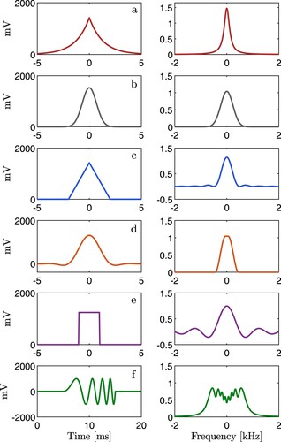
Figure 2. Energy spectral density of the two-sided decaying exponential, Gaussian, triangular, raised cosine, rectangular and rectangular chirp pulse.
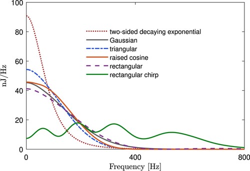
Table 1. Electromagnetic pulse parameters.
Table 2. Skin depth in D6ac steel and aluminium at different frequencies.
Figure 3. Electromagnetic pulse experiment setup. The cDAQ generates a voltage pulse in the transmitter coil, which creates a magnetic flux density that penetrates the metallic object and induces eddy currents. The eddy currents generate a magnetic flux density
transient that is detected by the receiver coil. The transient passes through the preamplifier and into a cDAQ analog-to-digital converter. The data is then recorded on the laptop.
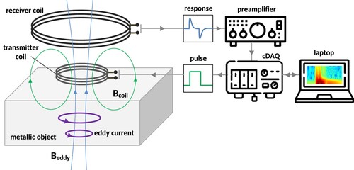
Figure 4. The eight metallic objects used in the experiment.
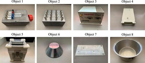
Figure 5. Illustration of the neural network model used in this work. The input to the neural network is the time signature of the scattering response of object 8 at 10 mm from the sensor system, and is generated by a two-sided decaying exponential pulse and contains 4000 data points. This is densely connected to layer 1 with 4096 neurons and a ReLU activation function, which is connected to layer 2 with 128 neurons and a ReLU activation function. Dropout of 0.2 is applied after layer 2 and densely connected to layer 3 containing 8 neurons with a softmax function. The metallic object is classified using an argmax function.
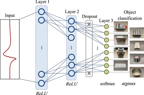
Figure 6. Illustration of the 1D CNN model used in this work. The input to the 1D CNN is the time signature of the scattering response of object 8 at 10 mm from the sensor system and generated by a two-sided decaying exponential pulse. Two 1D convolutional layers are used and these have the same properties – 16 filters of kernel size 64 with padding that ensures the input and output length remains constant at 4000 samples, and a ReLU activation function. These convolutional layers are stacked together and plotted as a surface in the illustration and are known as feature maps. In the feature maps red indicates large weight assigned by the 1D CNN and blue indicates small weight. The output from the second convolutional layer is flattened and densely connected to 8 neurons with a softmax activation function and the metallic object is classified using an argmax function.
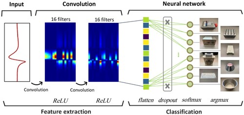
Figure 7. Illustration of the 2D CNN model used in this work. The input is a spectrogram of the scattering response of object 8 placed 10 mm from the sensor system and generated by a two-sided decaying exponential pulse. The input spectrogram has a 3 × 3 filter convolved over all pixels, and then max pooling of spatial size 2 × 2 is applied. The convolution using 3 × 3 and max pooling of 2 × 2 is repeated two times with ReLU activation functions on the output. The data is flattened and densely connected to 128 neurons with a ReLU activation function followed by dropout of 0.5. This is then connected to 8 neurons with a softmax function and finally an argmax function is applied to classify the metallic object.
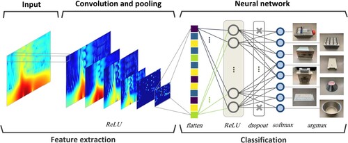
Figure 8. Receiver coil time signatures including reference, total, and scattered of object 1 at 10 mm for pulses (a) two-sided decaying exponential, (b) Gaussian, (c) triangular, (d) raised cosine, (e) rectangular and (f) rectangular chirp.
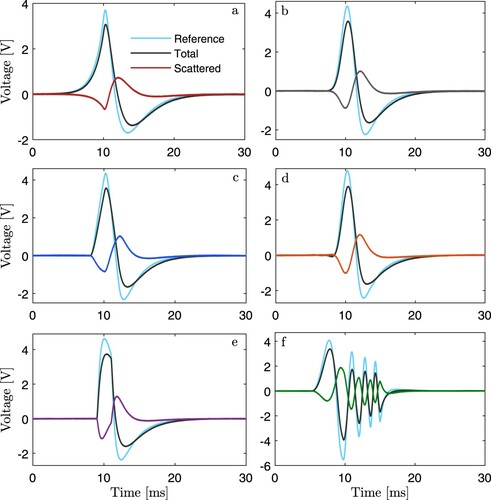
Figure 9. Receiver coil scattered time signatures of all objects at 10 mm, with spectrograms of object 8 to the right of the plot, for pulses (a) two-sided decaying exponential, (b) Gaussian, (c) triangular, (d) raised cosine, (e) rectangular and (f) rectangular chirp.
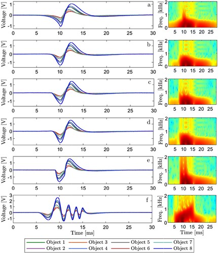
Figure 10. Object images, spectrograms, and electromagnetic scattered time signature data for the rectangular pulse. Spectrograms are expressed as power per frequency on a scale of dB/Hz to
dB/Hz. Objects are 10 mm from the sensor system.
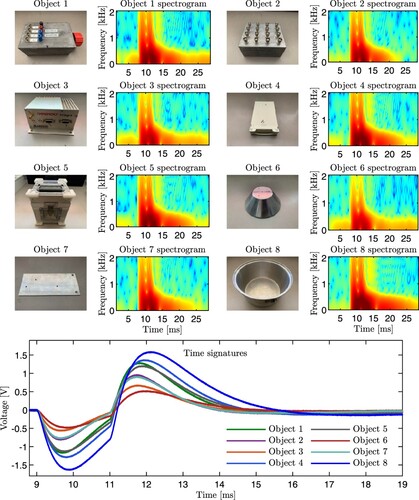
Figure 11. Machine learning classification results for each pulse and classifier. Each circle marker is a classification accuracy in the 10-fold cross-validation. The minimum, maximum, first quartile, third quartile, and median are also shown. Note that the perceptron has a different horizontal scale for illustration purposes.
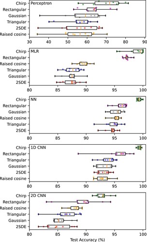
Figure 12. Mean classification accuracy and standard deviation (%) over 10-fold cross-validation for all pulses and classifiers.
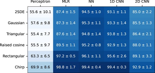
Figure 13. Dropout versus classification accuracy where bars are mean classification accuracy, error bars are the standard deviation, and circle markers indicate the classification accuracy of each fold in the 10-fold cross-validation.
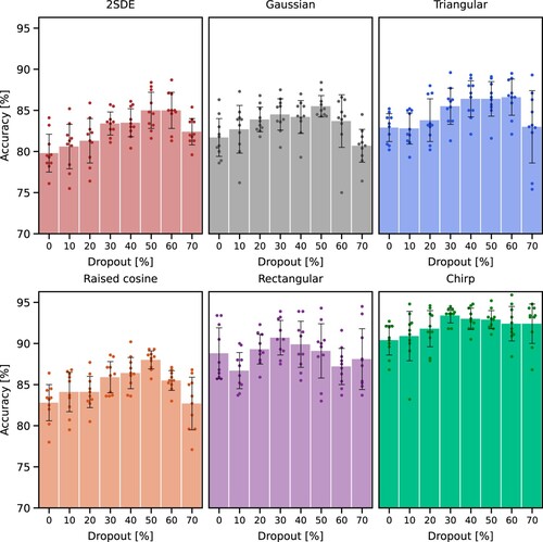
Figure 14. Confusion matrices of summed 10-folds for all pulses and classifiers.
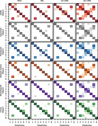
Figure 15. Receiver coil scattered time signatures of object 8 at 10 mm, and the first and second convolutional layer feature maps, for pulses (a) two-sided decaying exponential, (b) Gaussian, (c) triangular, (d) raised cosine, (e) rectangular and (f) rectangular chirp. In the feature maps red signifies large weight and blue signifies small weight in the 1D CNN.
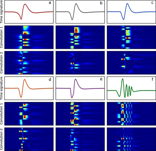
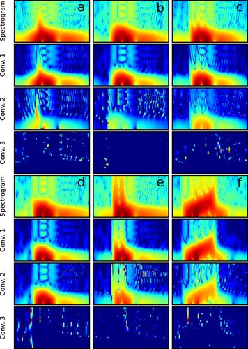
Figure 16. Spectrogram input and a subset of 2D CNN feature maps of convolutional layers for object 8 placed 10 mm above the sensor system for pulses: (a) two-sided decaying exponential, (b) Gaussian, (c) triangular, (d) raised cosine, (e) rectangular and (f) rectangular chirp. In the feature maps red signifies large weight and blue signifies small weight in the 2D CNN.