Defect phases – thermodynamics and impact on material properties

Figures & data

Figure 1. Defect phase diagrams as a potential new basis for materials design joining the current strategies of phase and defect engineering. An analogous picture could be drawn for Pourbaix diagrams and the interaction of corrosion mechanisms with defects.

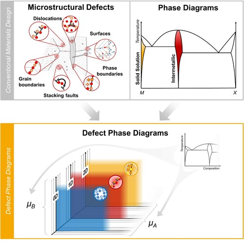
Figure 2. Defect in different states given by its chemical and structural atomic complexity. Left: ‘textbook’ symmetrical tilt boundary without chemical complexity. From middle to right: Increasing structural and chemical atomic complexity giving rise to different defect states or phases as a second atom species is added.

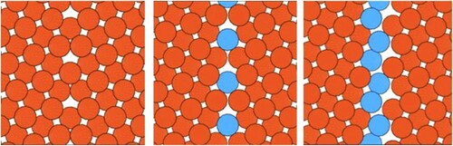
Table 1. Essential keywords in the context of defect phase diagrams.

	Definitions/examples
Defect type	Surface, phase boundary, grain boundary, dislocation
Defect character	Grain boundary character, surface orientation, e.g. (100) surface, or dislocation character, e.g. basal edge dislocation
Defect state	Specific atomic structure and chemistry at the defect
Defect phase	Stable and distinct defect state under certain thermodynamic variables

Table 2. Definitions of suitable ‘spaces’ connecting fundamental experiments, the underlying defect phase and the resulting engineering properties.

	Definition	Typical variables
Experimental space	Space in which the virtual and real experiments are conducted.	Temperature, composition, pH, stress, interatomic potential, etc.
µ-space	Space in which defect phase and mechanism-property diagrams are constructed.	Chemical potential
Engineering space	Space in which properties and conditions are combined for engineering design.	Temperature, composition, yield stress, fracture toughness, electro-chemical potential, etc.

Figure 3. Construction of defect phase diagrams using dislocations in intermetallic phases as an example. Theory and experiment work together synergistically to create defect phase diagrams.

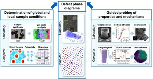
Figure 4. Continuous translation from experimental space to µ-space

to engineering space using the same example as above, dislocations in a hexagonal structure. The defect phase diagrams (DPDs) (µ-space) are connected with the mechanism maps (engineering space) via mechanism-property-diagrams (µ-space). The latter can be generated from the defect phases and their measured and computed properties and mechanisms (obtained by guided probing) to reflect a competition of choice between different mechanisms (here the competition between different slip systems and the resulting deformation behaviour).

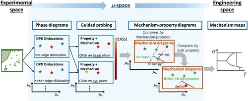
Figure 5. Visualisation of the complete framework linking all types of defect phase diagrams and defect phase properties from experimental space across µ-space to engineering space. DPD: defect phase diagram; µ: chemical potential.

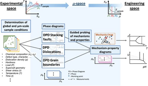
Figure 6. Schematic represerntation of the stages of defect equilibration: potential energy vs. reaction coordinate.

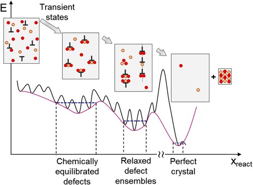
Figure 7. Selected approaches to visualise defect phase diagrams. (A) Experimental phase diagram for the Al₂O₃-Y₂O₃ system indicating stability regions of low T and high T complexions as well as their coexistence [18]. Computed diagrams for effective grain boundary (GB) width (GB λ diagram) in (B) the Mo-Ni [74] and (C) the W-Ni-Fe systems [73]. (D) Phase diagram of the Cu-Zr system highlighting the stability of ordered (yellow) and disordered (magenta) linear complexions as function of global and local composition [5]. (E) Phase diagram for the WC/Co interface where different stackings have been distinguished. The diagram is plotted as function of the chemical potential of cubic VC doping [119]. Images reprinted with permission from Elsevier, Wiley and the American Physical Society from A [18], B [74], C [73], D [5], E [119]. Reuse not permitted.

Figure 8. Combined defect and bulk phase diagram of Ni-H. The insets show the bulk and defect phases at the atomistic scale. The data for the bulk phase diagram are taken from [121] and for the defect phase diagram from [120].

Figure 9. Change in the Gibbs free energy with oxygen chemical potential for Pd surfaces in contact with an oxygen atmosphere. Red lines depict the respective surface phase diagrams.

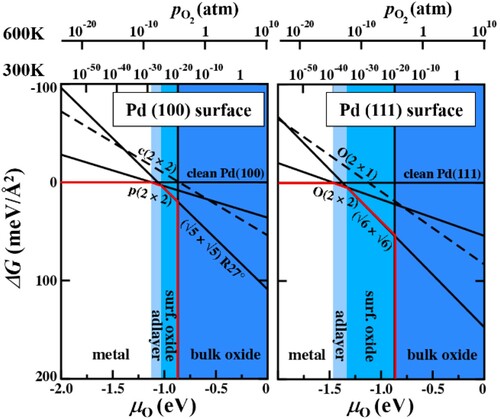
Figure 10. Surface phase diagrams for a ZnO(0001) surface in contact with a humid oxygen atmosphere. Differently coloured regions mark the stability regions of different surface reconstructions. The white dashed area indicates the region where water condensates at the surface. Geometries of the stable surface structures are shown as insets. Adapted from [133] with permission from the American Physical Society. Reuse not permitted.

Figure 11. Fe–9 atomic % Mn solid solution, 50% cold-rolled and annealed at 450°C for 6 h to trigger Mn segregation. (A) Bright-field STEM image. (B) Correlative atom probe tomography results of the same tip shown in (A) using 12.5 atomic % Mn isoconcentration surfaces (12.5 atomic % Mn was chosen as a threshold value to highlight Mn-enriched regions). The blue arrows mark grain boundaries and dislocation lines that are visible in both the STEM micrograph and the atom probe tomography map. Not all dislocations visible in STEM are also visible in the atom probe data and vice versa (red arrows). (C) Overlay of (A) and (B). (D) Magnification of two subregions taken from (B). (E) 1D compositional profiles along 1 (perpendicular to dislocation line) and 2 (along dislocation line). Reprinted with permission from AAAS, Ref. [3].Reuse not permitted.

Figure 12. Atom probe tomography analysis along Mn-decorated dislocation cores, revealing low-dimensional spinodal decomposition patterns along the dislocation lines. From Kwiatkowski et al. [134], published under a Creative Commons Attribution 4.0 license.

Figure 13. Yttrium-similarity index, YSI for the 2850 solute pairs computed in this study and visualised in the form of a symmetric matrix (a) with yellow indicating a high similarity and blue a low one. Solute pairs that have a high index (YSI>0.95) are shown in the upper triangular part in (b). Applying a cost and solubility filter only a single pair, Al-Ca, remains (c). From [141], published under a Creative Commons Attribution 4.0 International License by Springer Nature.

Figure 14. (a) Engineering stress-strain curves of the discussed Mg-Al-Ca alloy in comparison with not engineered (other than simple homogenisation treatment) solid solution Mg-Y, Mg-RE, pure Mg and Mg-Al-0.3Ca [141]. The inset shows the ultimate tensile strength – uniform elongation diagram of the same alloys displaying the superior mechanical properties of the alloy developed using the YSI. RD: rolling direction; TD: transverse direction. Compositions are in weight %. (b) Pure Mg fractured along macroscopic shear bands when cold rolled to 10% thickness reduction whereas Mg–1Al–0.1Ca could be cold rolled to 54% thickness reduction in several rolling passes of 8% thickness reduction per rolling pass; small sheet sections cut from the rolled sheet after each consecutive rolling pass are presented. From [141], published under a Creative Commons Attribution 4.0 International License by Springer Nature.

Figure 15. One- and two-dimensional examples of defects with structural and chemical atomic complexity in intermetallics, metals, oxides and carbide-metal composites observed in experiments (A–D) and simulations (E–H). Images in B and F reprinted from [180], published under a Creative Commons Attribution 4.0 International License. The other images are reprinted with permission from Elsevier from the following references: A [154], C [18], D [181], E [151], G [18], H [119]. Reuse not permitted.

Figure 16. Combination of experimental and computation nanomechanics enables scale-bridging study of deformation mechanisms in ordered crystals, which tend to be brittle at the macroscopic scale and low temperature, enabling the population of defect phase and mechanism-property diagrams in the future. Measurement of critical stresses for yielding (A) and energy barriers for different deformation mechanisms (F) from experimental (C) and computational (D) nanomechanical studies. Observation of both static and moving dislocations at the same level of resolution is made possible by HR-TEM (B) and molecular dynamics simulations (E). Images reprinted with permission from Elsevier and Wiley from references A [168], B [174], C [182], D [156], E [183], F [156]. Reuse not permitted.

Figure 17. (a) Atomic structures and energy surface for the $\left\{10\overline{1}2\right\}$ tensile twins in pure Mg. (b) Visualisation of the shear parameter $ϵ$ in units of half the Burgers vector $b$ and the shuffle parameter $s$ in units of the atomic plane distance $d$ describing the state of the TB. The energy minima correspond to the reflection TB ($ϵ=0,s=0$) and the glide TB ($ϵ=1,s=1$). The energies have been determined by an EAM potential. Figure adapted from Ref. [175], published under a Creative Commons Attribution 4.0 International License by Springer Nature.

Figure 18. (a) and (b) show the DOS available to dilutely segregating Mg atoms at (130) and (430) [001]$\mathrm{\Sigma }$5 Al GBs, respectively, calculated at 0 K with an empirical potential. Yellow (red) curves show Fermi-Dirac occupation of these states at 100 K (700 K). (c) and (d) ((e) and (f)) show the resulting structure predictions for these boundaries at low (high) temperature. Structures are projected onto the (001) plane and coloured according to Mg occupation probability (Al = grey, Mg = blue). For the disorderly (430) boundary, translucency is used to indicate atomic density in the [001] direction.

Figure 19. Coupled Molecular Dynamics/Monte Carlo simulations for Al-Mg at room temperature for increasing time/Monte Carlo steps. Positions are projected onto the (001) plane and grouped by column, with colour indicating species (grey = Al, blue = Mg). Red and yellow circles indicate areas of special interest (see text). Figure adapted from [179], published under a Creative Commons International 4.0 Attribution license.

Cantwell PR, Tang M, Dillon SJ, et al. Grain boundary complexions. Acta Mater. 2014;62:1–48.

 Web of Science ®Google Scholar

Shi X, Luo J. Developing grain boundary diagrams as a materials science tool: a case study of nickel-doped molybdenum. Phys Rev B. 2011;84(1):014105.

 Web of Science ®Google Scholar

Zhou N, Luo J. Developing grain boundary diagrams for multicomponent alloys. Acta Mater. 2015;91:202–216.

 Web of Science ®Google Scholar

Turlo V, Rupert TJ. Prediction of a wide variety of linear complexions in face centered cubic alloys. Acta Mater. 2020;185:129–141.

 Web of Science ®Google Scholar

Johansson SAE, Wahnström G. First-principles derived complexion diagrams for phase boundaries in doped cemented carbides. Curr Opin Solid State Mater Sci. 2016;20(5):299–307.

 Web of Science ®Google Scholar

Fukai Y, Yamatomo S, Harada S, et al. The phase diagram of the Ni· H system revisited. J Alloys Compd. 2004;372(1-2):L4–L5.

 Web of Science ®Google Scholar

Leyson G, Grabowski B, Neugebauer J. Multiscale description of dislocation induced nano-hydrides. Acta Mater. 2015;89:50–59.

 Web of Science ®Google Scholar

Valtiner M, Todorova M, Grundmeier V, et al. Temperature Stabilized Surface Reconstructions at Polar ZnO(0001). Phys. Rev. Lett. 2009;103(6):065502.

 Google Scholar

Kuzmina M, Herbig M, Ponge D, et al. Linear complexions: confined chemical and structural states at dislocations. Science. 2015;349(6252):1080–1083.

 PubMed Web of Science ®Google Scholar

Kwiatkowski da Silva A, Ponge D, Peng Z, et al. Phase nucleation through confined spinodal fluctuations at crystal defects evidenced in Fe-Mn alloys. Nat Commun. 2018;9(1):1137.

 PubMedGoogle Scholar

Sandlöbes S, Friák M, Korte-Kerzel S, et al. A rare-earth free magnesium alloy with improved intrinsic ductility. Sci Rep. 2017;7(1):10458.

 PubMed Web of Science ®Google Scholar

Yang Z, Zhang L, Chisholm MF, et al. Precipitation of binary quasicrystals along dislocations. Nat Commun. 2018;9(1):1–7.

 PubMedGoogle Scholar

Korte-Kerzel S, Schnabel V, Clegg WJ, et al. Room temperature plasticity in m-Al13Co4 studied by microcompression and high resolution scanning transmission electron microscopy. Scr Mater. 2018;146:327–330.

 Web of Science ®Google Scholar

Liu X, Song X, Wang H, et al. Complexions in WC-Co cemented carbides. Acta Mater. 2018;149:164–178.

 Web of Science ®Google Scholar

Heidelmann M, Heggen M, Dwyer C, et al. Comprehensive model of metadislocation movement in Al13Co4. Scr Mater. 2015;98:24–27.

 Web of Science ®Google Scholar

Schröders S, Sandlöbes S, Birke C, et al. Room temperature deformation in Fe7Mo6 µ-phase. Int J Plast. 2018;108:125–143.

 Web of Science ®Google Scholar

Schröders S, Sandlöbes S, Berkels B, et al. On the structure of defects in the Fe7Mo6 μ-phase. Acta Mater. 2019;167:257–266.

 Web of Science ®Google Scholar

Korte S, Clegg WJ. Studying plasticity in hard and soft Nb-Co intermetallics. Adv Eng Mater. 2012;14(11):991–997.

 Web of Science ®Google Scholar

Guénolé J, Mouhib F-Z, Huber L, et al. Basal slip in Laves phases: the synchroshear dislocation. Scr Mater. 2019;166:134–138.

 Web of Science ®Google Scholar

Guénolé J, Zubair M, Roy S, et al. Exploring the transfer of plasticity across Laves phase interfaces in a dual phase magnesium alloy. Mater Des. 2021;202:109572.

 Web of Science ®Google Scholar

Pei Z, Zhang X, Hickel T, et al. Atomic structures of twin boundaries in hexagonal close-packed metallic crystals with particular focus on Mg. NPJ Comput Mater. 2017;3(1):1–7.

 Google Scholar

Zhao H, Huber L, Lu W, et al. Interplay of chemistry and faceting at grain boundaries in a model Al Alloy. Phys Rev Lett. 2020;124(10):106102.

 PubMed Web of Science ®Google Scholar