A unified dynamic neural field model of goal directed eye movements

Figures & data

Figure 1. Different neural field models used to detect and track a moving target. The original DNF equation may converge on a limit cycle attractor in presence of the target, yet lagging behind it. On the contrary, the projections of the PNF version allows to converge and synchronise with the target motion. If the target crosses the visual field, only the ANF version is able to smoothly track the target, thus mimicking the dynamics of the brain–body-environment system through visuomotor interactions.

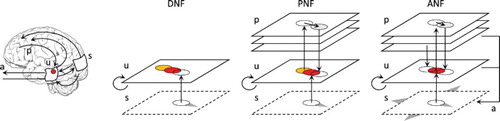
Table 1. Parameters and variables of the neural field model.

Group of parameters	Description	Symbol	Value/space
Visual field
	Visual field space	$\mathit{X}$	$[-0.5,0.5{]}^2$
	Coordinates within the field	$\mathit{x}$	$\in \mathit{X}$
	Field coordinates (world reference frame)	${\mathit{x}}_{\mathit{f}}$	$\in {\mathbb{R}}^2$
Neural field equation/potential		$\mathit{u}$	$\mathit{X}\to [0,1]$
	Time constant	τ	0.2
	Resting potential	h	0
	Firing/activation function (ReLU)	f	$\mathbb{R}\to {\mathbb{R}}^{+}$
	Stimulation/projection coefficient	α	0.5
	Focus coordinates (peak centre)	${\mathit{x}}_{\mathit{u}}$	$\in \mathit{X}$
Lateral connectivity kernel		$\mathit{w}$	$\mathit{X}\to [-1,1]$
	Excitatory amplitude	$A_{+}$	0.06
	Excitatory range (sd)	${\sigma }_{+}$	0.1
	Inhibitory amplitude	$A_{-}$	0.03
	Excitatory range (sd)	${\sigma }_{-}$	1.0
Gaussian stimulus		$\mathit{s}$	$\mathit{X}\to [0,1]$
	Stimulation amplitude	$A_s$	$\in \{0,1\}$
	Stimulation range (sd)	${\sigma }_s$	0.1
	Stimulus noise (white)	$\mathit{ϵ}$	$\mathit{X}\to \mathbb{R}$
	Noise amplitude (sd)	${\sigma }_{ϵ}$	0.2
	Stimulus velocity	${\mathit{v}}_{\mathit{s}}$	$\in [-3,3{]}^2$
	Stimulus location (field reference frame)	${\mathit{x}}_{\mathit{s}}$	$\in \mathit{X}$
	Stimulus location (world reference frame)	${\hat{\mathit{x}}}_{\mathit{s}}$	$\in {\mathbb{R}}^2$
Projection(s)		${\mathit{p}}_{\mathit{k}}$	$\mathit{X}\to [-1,1]$
	Projection weight (validity)	$w_k$	$\in [0,1]$
	Projection “velocity”	${\mathit{v}}_{\mathit{k}}$	$\in [-5,5{]}^2$
Eye movement
	Motor space	$\mathit{A}$	$[-1,1{]}^2$
	Motor command	$\mathit{a}$	$\mathit{A}$
	Induced spatial displacement	${\mathit{x}}_{\mathit{a}}$	$[-1,1{]}^2$
	Associated projection	${\mathit{p}}_{\mathit{a}}$	$\mathit{X}\to [-1,1]$
	Activation threshold	$u_a$	0.4
Discretisation/dynamics
	Time	t	$\in \mathbb{R}$
	Time step	$\mathrm{d}t$	0.05
	Spatial resolution	n	51

Figure 2. Illustration of the neural field model dynamics and equation components. For each model, stimulation at time $t-\mathrm{d}t$ (light colour on first row) and t (dark colour on first row), field activity from $t-\mathrm{d}t$ (light colour on third row) and resulting at t (dark colour on third row), as well as the competition component (negative activity on second row), are represented. Internal input projections corresponding to expected trajectories are also shown for the PNF and ANF models. With a moving stimulus, the DNF model is not able to converge to a stable peak of maximal activity, the peak lagging behind the target and/or decaying. The projection of activity in the PNF model simply compensates for the inertia of the equation and synchronises with the target trajectory (if the implicit expectation and observation match). The ANF model additionally includes a projection due to the eye movement, thus cancelling the drifting effect of the projection when the target image is kept within the central visual field.

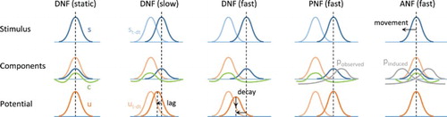
Figure 3. Architecture of the ANF model. The model first includes the lateral interaction ($\mathit{c}$) and integration of input stimulation ($\mathit{s}$) from the DNF model. It also integrates the projections (${\mathit{p}}_{\mathit{k}}$ with weight $w_k$) from the PNF model, themselves evaluated based on their ability to predict the current (here-and-now) location of the target (${\hat{\mathit{p}}}_{\mathit{k}}$). In addition, the model also controls eye movements (a), and thus can predict the associated transformations on the visual field to be facilitated by a projection of activity (${\mathit{p}}_{\mathit{a}}$) on the neural field. At each simulation time step, all components are combined with the neural field potential $\mathit{u}\left(t\right)$ to produce $\mathit{u}(t+\mathrm{d}t)$.

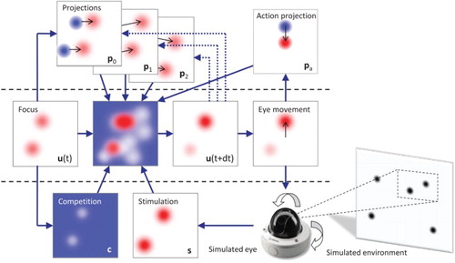
Table 2. Tracking statistics and their interpretation based on the type of target dynamics.

	Tracking error	Nb of saccades	Behaviour
Target dynamics	$\overline{d_e}$	$\sum _t{a}_{\mathrm{saccade}}\left(t\right)$	interpretation
(all)	High	High	Random saccades (depending on noise/parameters)
Saltatory movement	Low	Low	Stable fixation on target
–	Low	High	Micro-saccades around target
–	High	Low	Continuous drift away from target
Smooth movement	Low	Low	A few catch-up saccades followed by smooth pursuit
–	Low	High	Catch-up saccades during the entire simulation
–	Medium	Medium	Alternation of fixations and saccades
–	High	Low	Target lost during the simulation

Figure 4. Representative trajectory of the Cartesian visual field coordinates in the environment, when focusing on targets adopting a new random position every second. The left figure reflects the relative complexity of the trajectory, with a sequence of saccades and fixations matching the stimulus dynamics, but also random fluctuations and micro-saccades. The right figure displays the power spectrum of the movements along the x-axis, with a decreasing. (a) Simulated eye position along the x-axis and (b) Power spectrum of the movements along the x-axis.

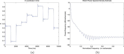
Figure 5. Distance between the visual field centre and actual target coordinates ($d_e$) as a function of time, for a system with a null projected velocity (${\mathit{v}}_{\mathit{k}}=\mathbf{0}$) and targets moving along a rectilinear trajectory at various speeds ($\parallel {\mathit{v}}_{\mathit{s}}\parallel \in \{0,.5,1,1.5,2,2.5\}$). This allows testing the behaviour of the original DNF model endowed with the ability to generate of eye movements. All stimuli are designed to reach the centre of the visual field at t=0 in absence of eye movements. Dotted lines correspond to the extrapolated target trajectories in the field reference frame, where no eye movement would be performed. For small increasing speeds, the target is detected and tracked with an increasing lag. For larger amplitudes, the target is captured and tracked through sequences of catch-up saccades. For extreme increasing speeds, the target gets lost sooner, or not even detected (for $\parallel {\mathit{v}}_{\mathit{k}}\parallel =2.5$). Values increasing beyond .5 betray a loss of target (i.e. target exiting the visual field that cannot be captured again).

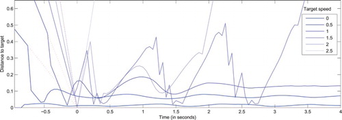
Figure 6. Distance between the visual field centre and actual target coordinates ($d_e$) as a function of time, for a system presented with targets moving along a rectilinear trajectory with a constant speed ($\parallel {\mathit{v}}_{\mathit{s}}\parallel =2$), but with different projected velocities, all matching the motion direction of the target, but with different amplitudes ($\parallel {\mathit{v}}_{\mathit{k}}\parallel \in \{0,.5,1.5,2.5\}$). All stimuli are designed to reach the centre of the visual field at t=0 in absence of eye movements. As the projected speed gets closer to its optimal value, fewer catch-up saccades are performed, and the target is tracked with a diminishing lag. As discussed in the main text and in order to correctly estimate the validity of projections, the lag is never fully cancelled.

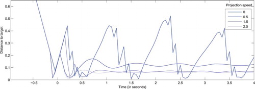
Figure 7. Mean distance between the simulated eye and real target coordinates after t=0 (colour gradient) and average number of saccades per trial (figures), for a target moving at $\parallel {\mathit{v}}_{\mathit{s}}\parallel =2$ units/second along the horizontal axis ($1\mathrm{unit}=\mathrm{visual}\mathrm{field}\mathrm{width}$). Each cell corresponds to 200 simulations of the system running with a single projection, with the corresponding projection velocity components indicated along the axes. A bell-shaped profile appears around the target speed coordinates (with low error, and less than 2 catch-up saccades to capture the target), reflecting the discrimination capabilities of the projections.

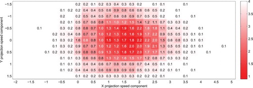
Figure 8. Mean distance between the simulated eye and real target coordinates after t=0 (colour gradient) and average number of saccades per trial (figures), for a target moving at different speeds and for various projection speeds (both velocity vectors remaining collinear). Each cell corresponds to 200 simulations of the system running with a single projection, with the target and projection speed values indicated along the axes.

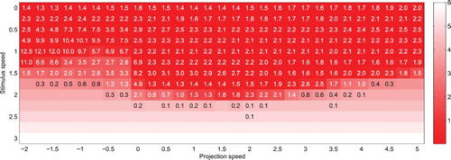
Figure 9. Illustration of the ANF model dynamics in presence of a moving target following a rectilinear trajectory with constant speed. Adopted states and transitions depend on the target dynamics and internal projection of activity, and are thus implicitly represented here using arrows: low or compatible speeds with single-headed arrows, high speeds and/or medium discrepancy with double-headed arrows, extreme speeds or high discrepancy with triple-headed arrow. Apparent target position in the visual field is represented as a dashed circle while the neural field peak is represented by a Gaussian profile activity whose intensity reflects the peak amplitude. Please refer to the main text for the detailed description of the labelled transitions.

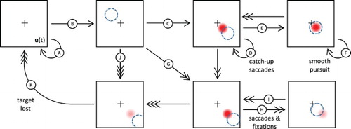
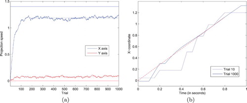
Figure 10. Illustration of the learning dynamics of the ANF system when updating the projection of activity on the neural field after each trials, reproducing experimental data from Bourrelly et al. (2016). (a) The projection speed components (X and Y) rapidly converge to relatively stable values (dashed lines for the asymptotic means), yet different from the target speed components (plain lines at 1.4 for X, and 0 for Y), due to the complex neural field dynamics. (b) Representative trajectories for trials #10 and #1000. The behaviour drastically changes, with an earlier capture of the target, a reduction in the number of catch-up saccades, the dominance of smooth pursuit, and the continuing tracking at the here-and-now position of the target even after its disappearance (dashed line corresponding to the target trajectory, and stopping at t=.8 s). (a) Convergence of the “projection speed” and (b) Trajectory samples before/after learning.

Table 3. Performance statistics for representative trials during learning.

Run	#10	#1000
Mean peak eccentricity ($\overline{\parallel x_u\parallel }$)	0.193	0.070
Mean tracking error ($\overline{d_e}$)	0.085	0.027
Number of saccades ($\sum a_{\mathrm{saccade}}$)	5	2

Bourrelly, C., Quinet, J., Cavanagh, P., & Goffart, L. (2016). Learning the trajectory of a moving visual target and evolution of its tracking in the monkey. Journal of Neurophysiology, 116(6), 2739–2751. doi: 10.1152/jn.00519.2016

 PubMed Web of Science ®Google Scholar