Significance of eigenstresses and curling stresses for total thermal stresses in a concrete slab, as a function of subgrade stiffness

Figures & data

Figure 1. Field testing site: (a) cuts hosting the temperature sensors and their cables, (b) condition after closing the cuts with a resin, and (c) vertical positions of the sensors.

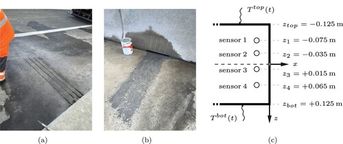
Table 1. Geometric dimensions of the studied pavement slab and material properties of concrete; values taken from Wang et al. (2019a) are estimates from multiscale modelling, accounting for corresponding properties of cement paste and aggregates.

Property	Value	Source
Length of the slab	$l_x=5.50\mathrm{m}$
Width of the slab	$l_y=2.70\mathrm{m}$
Thickness of the slab	$h=0.25\mathrm{m}$
Thermal diffusivity	$a=1.4\times {10}^{-6}{\mathrm{m}}^2/\mathrm{s}$	Equation (13(13) $a=1.4\times {10}^{-6}{\mathrm{m}}^2/\mathrm{s}.$(13) )
Coefficient of thermal expansion	${\alpha }_T=1.153\times {10}^{-5}{/}^{\circ }\mathrm{C}$	(Wang et al. 2019a)
Modulus of elasticity	$E=31.76\mathrm{GPa}$	(Wang et al. 2019a)
Poisson's ratio	$\nu =0.203$	(Wang et al. 2019a)
Mass density	$\rho =2,400\mathrm{kg}/{\mathrm{m}}^3$

Figure 2. Temperatures measured $5\mathrm{cm}$, $9\mathrm{cm}$, $14\mathrm{cm}$ and $19\mathrm{cm}$ underneath the top surface, from 1 Oct. to 8 Oct.; for the complete database, see Appendix 2; both 7 and 8 Oct. were foggy days with a quite stable temperature, see (Time 2020).

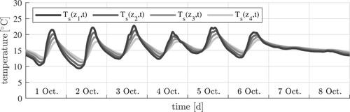
Figure 3. Representation of the temperature histories at the top and the bottom of the plate by means of step functions, starting from the initial temperatures $T_{ini}^{top}$ and $T_{ini}^{bot}$, respectively.

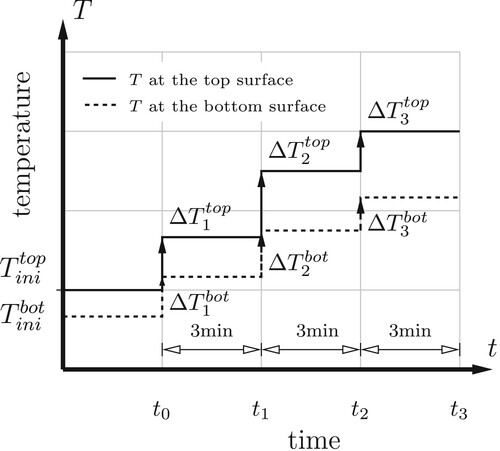
Figure 4. Spatial extrapolation of temperatures referring to the positions of the four PT100A sensors, see the circles, to the top and the bottom of the plate, see the squares, using the best-fit quadratic polynomial according to Equation (7(7) $T(z,t)=A_0(t)+A_1(t)\cdot \frac{z}{h}+A_2(t)\cdot {\left(\frac{z}{h}\right)}^2,$(7) ), see also Table 2.

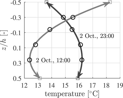
Table 2. Coordinates of the sensors and of the top and the bottom of the slab; thickness of the slab; optimal coefficients of best-fit quadratic polynomials (7(7) $T(z,t)=A_0(t)+A_1(t)\cdot \frac{z}{h}+A_2(t)\cdot {\left(\frac{z}{h}\right)}^2,$(7) ); and resulting extrapolation formulae for quantification of the temperature at the top and the bottom of the plate.

z-coordinates of the sensors, the top and the bottom of the slab, and its thickness
$z_1=-0.075\mathrm{m}$, $z_2=-0.035\mathrm{m}$, $z_3=+0.015\mathrm{m}$, $z_4=+0.065\mathrm{m}$
$z_{top}=-0.125\mathrm{m}$, $z_{bot}=+0.125\mathrm{m}$; $h=0.25\mathrm{m}$
Optimal coefficients of the quadratic fitting function (7(7) $T(z,t)=A_0(t)+A_1(t)\cdot \frac{z}{h}+A_2(t)\cdot {\left(\frac{z}{h}\right)}^2,$(7) )
$A_0(t)=-0.12592T_s(z_1,t)+0.51231T_s(z_2,t)+0.62795T_s(z_3,t)-0.01434T_s(z_4,t)$
$A_1(t)=-1.24783T_s(z_1,t)-0.85548T_s(z_2,t)+0.20487T_s(z_3,t)+1.89844T_s(z_4,t)$
$A_2(t)=+7.48851T_s(z_1,t)-6.37106T_s(z_2,t)-8.22573T_s(z_3,t)+7.10827T_s(z_4,t)$
Formulae providing spatial extrapolation of temperatures to the top and the bottom of the plate
$T^{top}(t)=T(z_{top},t)=+2.37013T_s(z_1,t)-0.65272T_s(z_2,t)-1.53092T_s(z_3,t)+0.81351T_s(z_4,t)$
$T^{bot}(t)=T(z_{bot},t)=+1.12230T_s(z_1,t)-1.50819T_s(z_2,t)-1.32605T_s(z_3,t)+2.71194T_s(z_4,t)$

Figure 5. Boundary conditions of the transient heat conduction problem: evolution of temperatures at the top and the bottom of the plate, obtained with the extrapolation function (7(7) $T(z,t)=A_0(t)+A_1(t)\cdot \frac{z}{h}+A_2(t)\cdot {\left(\frac{z}{h}\right)}^2,$(7) ); the data shown refer to 1 Oct. to 8 Oct.

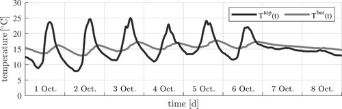
Figure 6. Temperature profiles referring to 2 Oct.: the circles label measured temperatures, the solid lines refer to the solution of the heat conduction problem according to Equation (8(8) $\begin{array}{rl}T(z,t)& =\frac{T^{bot}(t)+T^{top}(t)}{2}+[T^{bot}(t)-T^{top}(t)]\frac{z}{h}\\ & -\sum _{i=1}^{N_i}(\mathrm{\Delta }{T}_i^{top}-\mathrm{\Delta }{T}_i^{bot})\sum _{n=1}^{\mathrm{\infty }}\frac{(-1{)}^n}{n\pi }\sin \left(\frac{2n\pi z}{h}\right)\\ & \exp (-(2n\pi {)}^2\frac{a⟨t-t_i⟩}{h^2})+\sum _{i=1}^{N_i}(\mathrm{\Delta }{T}_i^{top}+\mathrm{\Delta }{T}_i^{bot})\\ & \sum _{n=1}^{\mathrm{\infty }}\frac{2(-1{)}^n}{(2n-1)\pi }\cos \left(\frac{(2n-1)\pi z}{h}\right)\\ & \exp (-(2n-1{)}^2{\pi }^2\frac{a⟨t-t_i⟩}{h^2}),\end{array}$(8) ), using the surface temperature histories of Figure 5 as boundary conditions.

Figure 7. Decomposition of thermal eigenstrains into (i) a spatially constant part, ${\epsilon }^e$, equal to the eigenstretch of the plate, (ii) a spatially linear part, ${\kappa }^e\cdot z$, related to the eigencurvature of the plate, and (iii) the spatially nonlinear rest, representing the eigendistortion ${\epsilon }_{dist}^e$ of the generators of the plate.

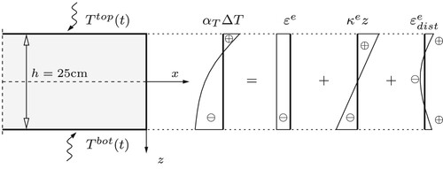
Figure 8. Exemplary results of thermo-elastic analysis: Decomposition of (a) the thermal eigenstrains into (b) eigenstrains referring to eigenstretches ${\epsilon }^e$ of the plate, (c) eigenstrains referring to eigencurvatures ${\kappa }^e$ of the plate (these eigenstrains are equal to the product of eigencurvatures ${\kappa }^e$ and the z-coordinate), and (d) eigenstrains referring to eigendistortions ${\epsilon }_{dist}^e$ of the generators of the plate; the results have shown refer to 2 Oct.

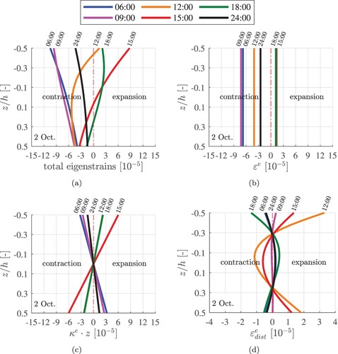
Table 3. Expressions for eigenstretches and eigencurvatures of the plate and for the eigendistortion of the generators of the plate, obtained from inserting the solution of the heat equation according to Equation (8(8) $\begin{array}{rl}T(z,t)& =\frac{T^{bot}(t)+T^{top}(t)}{2}+[T^{bot}(t)-T^{top}(t)]\frac{z}{h}\\ & -\sum _{i=1}^{N_i}(\mathrm{\Delta }{T}_i^{top}-\mathrm{\Delta }{T}_i^{bot})\sum _{n=1}^{\mathrm{\infty }}\frac{(-1{)}^n}{n\pi }\sin \left(\frac{2n\pi z}{h}\right)\\ & \exp (-(2n\pi {)}^2\frac{a⟨t-t_i⟩}{h^2})+\sum _{i=1}^{N_i}(\mathrm{\Delta }{T}_i^{top}+\mathrm{\Delta }{T}_i^{bot})\\ & \sum _{n=1}^{\mathrm{\infty }}\frac{2(-1{)}^n}{(2n-1)\pi }\cos \left(\frac{(2n-1)\pi z}{h}\right)\\ & \exp (-(2n-1{)}^2{\pi }^2\frac{a⟨t-t_i⟩}{h^2}),\end{array}$(8) ) into Equation (16(16) $\mathrm{\Delta }T(z,t)=T(z,t)-T_{ref},$(16) ), the resulting expressions into Equation (15(15) ${\epsilon }_{xx}^e(z,t)={\epsilon }_{yy}^e(z,t)={\epsilon }_{zz}^e(z,t)={\alpha }_T\mathrm{\Delta }T(z,t),$(15) ), and the obtained results into Equations (17(17) ${\epsilon }^e(t)=\frac{1}{h}\underset{-\frac{h}{2}}{\overset{+\frac{h}{2}}{\int }}{\alpha }_T\mathrm{\Delta }T(z,t)\mathrm{d}z,$(17) ), (18(18) ${\kappa }^e(t)=\frac{12}{h^3}\underset{-\frac{h}{2}}{\overset{+\frac{h}{2}}{\int }}{\alpha }_T\mathrm{\Delta }T(z,t)\cdot z\mathrm{d}z.$(18) ), and (19(19) ${\epsilon }_{dist}^e(z,t)={\alpha }_T\mathrm{\Delta }T(z,t)-{\epsilon }^e(t)-{\kappa }^e(t)\cdot z,$(19) ).

	Solution of the heat conduction problem according to Equation (8(8) $\begin{array}{rl}T(z,t)& =\frac{T^{bot}(t)+T^{top}(t)}{2}+[T^{bot}(t)-T^{top}(t)]\frac{z}{h}\\ & -\sum _{i=1}^{N_i}(\mathrm{\Delta }{T}_i^{top}-\mathrm{\Delta }{T}_i^{bot})\sum _{n=1}^{\mathrm{\infty }}\frac{(-1{)}^n}{n\pi }\sin \left(\frac{2n\pi z}{h}\right)\\ & \exp (-(2n\pi {)}^2\frac{a⟨t-t_i⟩}{h^2})+\sum _{i=1}^{N_i}(\mathrm{\Delta }{T}_i^{top}+\mathrm{\Delta }{T}_i^{bot})\\ & \sum _{n=1}^{\mathrm{\infty }}\frac{2(-1{)}^n}{(2n-1)\pi }\cos \left(\frac{(2n-1)\pi z}{h}\right)\\ & \exp (-(2n-1{)}^2{\pi }^2\frac{a⟨t-t_i⟩}{h^2}),\end{array}$(8) ),
	using the surface temperature histories of Figure 5 as boundary conditions
	$\begin{array}{cc}{\epsilon }^e(t)& ={\alpha }_T(\frac{T^{bot}(t)+T^{top}(t)}{2}-T_{ref})\\ & -\sum _{i=1}^{N_i}{\alpha }_T\left(\frac{\mathrm{\Delta }{T}_i^{bot}+\mathrm{\Delta }{T}_i^{top}}{2}\right)\sum _{n=1}^{\mathrm{\infty }}\frac{8}{(2n-1{)}^2{\pi }^2}\exp (-(2n-1{)}^2{\pi }^2\frac{a⟨t-t_i⟩}{h^2})\\ {\kappa }^e(t)& ={\displaystyle \frac{{\alpha }_T}{h}[T^{bot}(t)-T^{top}(t)]}\\ & -\sum _{i=1}^{N_i}\frac{{\alpha }_T}{h}(\mathrm{\Delta }{T}_i^{bot}-\mathrm{\Delta }{T}_i^{top})\sum _{n=1}^{\mathrm{\infty }}\frac{24}{(2n\pi {)}^2}\exp (-(2n\pi {)}^2\frac{a⟨t-t_i⟩}{h^2})\end{array}$
	${\epsilon }_{dist}^e(z,t)$ follows from insertion of ${\alpha }_T\mathrm{\Delta }T(z,t)$ according to Equations (15(15) ${\epsilon }_{xx}^e(z,t)={\epsilon }_{yy}^e(z,t)={\epsilon }_{zz}^e(z,t)={\alpha }_T\mathrm{\Delta }T(z,t),$(15) ), (16(16) $\mathrm{\Delta }T(z,t)=T(z,t)-T_{ref},$(16) ), and (8(8) $\begin{array}{rl}T(z,t)& =\frac{T^{bot}(t)+T^{top}(t)}{2}+[T^{bot}(t)-T^{top}(t)]\frac{z}{h}\\ & -\sum _{i=1}^{N_i}(\mathrm{\Delta }{T}_i^{top}-\mathrm{\Delta }{T}_i^{bot})\sum _{n=1}^{\mathrm{\infty }}\frac{(-1{)}^n}{n\pi }\sin \left(\frac{2n\pi z}{h}\right)\\ & \exp (-(2n\pi {)}^2\frac{a⟨t-t_i⟩}{h^2})+\sum _{i=1}^{N_i}(\mathrm{\Delta }{T}_i^{top}+\mathrm{\Delta }{T}_i^{bot})\\ & \sum _{n=1}^{\mathrm{\infty }}\frac{2(-1{)}^n}{(2n-1)\pi }\cos \left(\frac{(2n-1)\pi z}{h}\right)\\ & \exp (-(2n-1{)}^2{\pi }^2\frac{a⟨t-t_i⟩}{h^2}),\end{array}$(8) )
	as well as ${\epsilon }^e(t)$ and ${\kappa }^e(t)$, see the expressions above, into Equation (19(19) ${\epsilon }_{dist}^e(z,t)={\alpha }_T\mathrm{\Delta }T(z,t)-{\epsilon }^e(t)-{\kappa }^e(t)\cdot z,$(19) ).

Figure 9. Structural model of a pavement slab: a rectangular plate with free edges rests on a Winkler foundation.

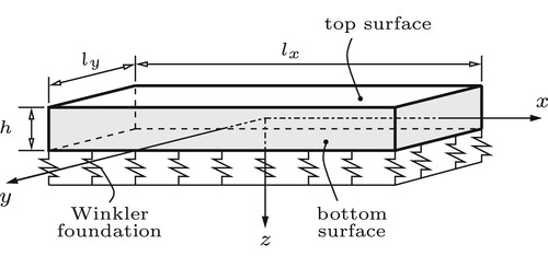
Figure 10. Exemplary results from nonlinear FE analyses: deformed configurations of plates subjected to (a) positive eigencurvature ${\kappa }^e=+2.6\times {10}^{-4}/\mathrm{m}$, resulting in concave curling, and (b) negative eigencurvature ${\kappa }^e=-4.8\times {10}^{-4}/\mathrm{m}$, resulting in convex curling; the modulus of subgrade reaction amounts to $100\mathrm{MPa}/\mathrm{m}$; these two values of the eigencurvature correspond to temperature gradients amounting to $-0.0225{}^{\circ }\mathrm{C}/\mathrm{mm}$ and $+0.0416{}^{\circ }\mathrm{C}/\mathrm{mm}$, i.e. to temperature differences between the top and the bottom of the plate amounting to $-{5.6}^{\circ }$C and $+{10.4}^{\circ }$C, respectively.

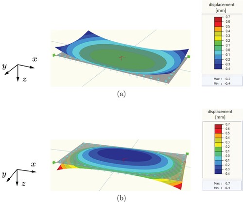
Figure 11. Results from nonlinear FE analyses: largest principal tensile curling stress as a function of the eigencurvature ${\kappa }^e$ and the modulus of subgrade reaction; the markers label numerical results (see Table 4 for numerical values), the lines are splines reproducing the simulation results and interpolating between them.

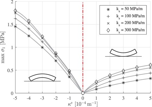
Table 4. Results from nonlinear FE analyses: largest principal tensile curling stress as a function of the eigencurvature ${\kappa }^e$ and the modulus of subgrade reaction $k_s$.

	$k_s=50$	$k_s=100$	$k_s=200$	$k_s=300$
	$\mathrm{MPa}/\mathrm{m}$	$\mathrm{MPa}/\mathrm{m}$	$\mathrm{MPa}/\mathrm{m}$	$\mathrm{MPa}/\mathrm{m}$
${\kappa }^e=-5\times {10}^{-4}/\mathrm{m}$	$1.453\mathrm{MPa}$	$1.627\mathrm{MPa}$	$1.748\mathrm{MPa}$	$1.800\mathrm{MPa}$
${\kappa }^e=-4\times {10}^{-4}/\mathrm{m}$	$1.248\mathrm{MPa}$	$1.404\mathrm{MPa}$	$1.520\mathrm{MPa}$	$1.574\mathrm{MPa}$
${\kappa }^e=-3\times {10}^{-4}/\mathrm{m}$	$0.997\mathrm{MPa}$	$1.171\mathrm{MPa}$	$1.200\mathrm{MPa}$	$1.233\mathrm{MPa}$
${\kappa }^e=-2\times {10}^{-4}/\mathrm{m}$	$0.706\mathrm{MPa}$	$0.801\mathrm{MPa}$	$0.849\mathrm{MPa}$	$0.866\mathrm{MPa}$
${\kappa }^e=-1\times {10}^{-4}/\mathrm{m}$	$0.354\mathrm{MPa}$	$0.422\mathrm{MPa}$	$0.467\mathrm{MPa}$	$0.481\mathrm{MPa}$
${\kappa }^e=+1\times {10}^{-4}/\mathrm{m}$	$0.086\mathrm{MPa}$	$0.140\mathrm{MPa}$	$0.210\mathrm{MPa}$	$0.247\mathrm{MPa}$
${\kappa }^e=+2\times {10}^{-4}/\mathrm{m}$	$0.163\mathrm{MPa}$	$0.253\mathrm{MPa}$	$0.341\mathrm{MPa}$	$0.387\mathrm{MPa}$
${\kappa }^e=+3\times {10}^{-4}/\mathrm{m}$	$0.226\mathrm{MPa}$	$0.333\mathrm{MPa}$	$0.433\mathrm{MPa}$	$0.487\mathrm{MPa}$
${\kappa }^e=+4\times {10}^{-4}/\mathrm{m}$	$0.278\mathrm{MPa}$	$0.392\mathrm{MPa}$	$0.501\mathrm{MPa}$	$0.561\mathrm{MPa}$
${\kappa }^e=+5\times {10}^{-4}/\mathrm{m}$	$0.320\mathrm{MPa}$	$0.438\mathrm{MPa}$	$0.551\mathrm{MPa}$	$0.614\mathrm{MPa}$

Table 5. Numerical results of maximum tensile curling stresses at the top and the bottom of the slab prescribing the largest and smallest eigencurvature of the entire monitoring period and different moduli of subgrade reaction.

$k_s$	$max{\sigma }_T({\kappa }^e)$[MPa]	$max{\sigma }_T({\kappa }^e)$[MPa]
$[\mathrm{MPa}/\mathrm{m}]$	top of slab	bottom of slab
50	0.20	1.42
100	0.31	1.60
200	0.40	1.72
300	0.45	1.77

Figure 12. Exemplary results of thermo-elastic analysis: curling stress distributions through the thickness of the slab, evaluated at six time instants of 2 Oct., computed with $k_s=100\mathrm{MPa}/\mathrm{m}$.

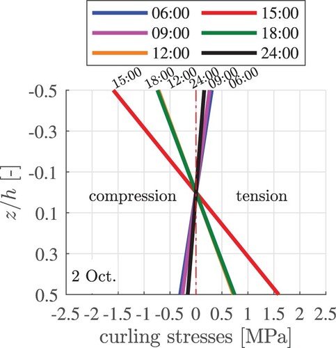
Figure 13. Exemplary results of thermo-elastic analysis: evolution of curling stresses at the top and the bottom of the slab on 2 Oct., computed with different moduli of subgrade reaction: the red markers label the maximum tensile curling stresses at the top and the bottom of the slab, in the corner regions and the central region, respectively.

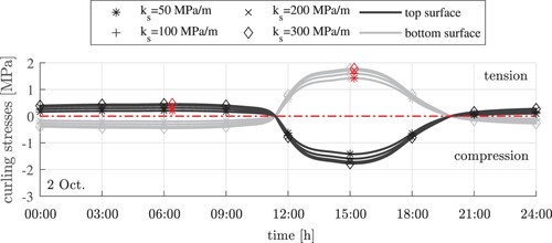
Figure 14. Exemplary results of thermo-elastic analysis: thermal eigenstress distributions through the thickness of the slab, evaluated at six time instants of 2 Oct.

Figure 15. Exemplary results of thermo-elastic analysis: thermal eigenstresses at the top, the midplane, and the bottom of the slab on 2 Oct.: the red markers label the maximum tensile eigenstresses.

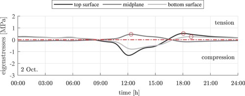
Figure 16. Exemplary results of thermo-elastic analysis: evolution of total thermal stress distributions through the thickness of the slab, evaluated at six-time instants of 2 Oct., computed with $k_s=100\mathrm{MPa}/\mathrm{m}$.

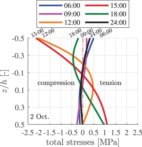
Figure 17. Exemplary results of thermo-elastic analysis: total thermal stresses at the top, the midplane, and the bottom of the slab on 2 Oct., computed with different moduli of subgrade reaction: the red markers label the maximum tensile curling stresses at the three different locations.

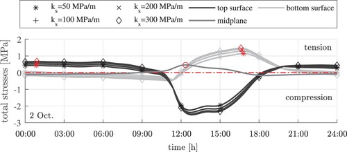
Table 6. Daily tensile stress maxima at the top of the slab: curling stresses and total thermal stresses, evaluated for four different values of the modulus of subgrade reaction.

	daily tensile curling stress maximum [MPa]				daily tensile total stress maximum [MPa]
$k_s$[MPa/m]	50	100	200	300	50	100	200	300
24 Sept.	0.16	0.25	0.34	0.38	0.25	0.34	0.43	0.48
25 Sept.	0.12	0.19	0.27	0.31	0.27	0.33	0.41	0.45
26 Sept.	0.09	0.15	0.22	0.26	0.26	0.31	0.37	0.41
27 Sept.	0.12	0.20	0.28	0.32	0.35	0.35	0.43	0.48
28 Sept.	0.14	0.23	0.31	0.36	0.48	0.51	0.57	0.61
29 Sept.	0.18	0.27	0.36	0.41	0.38	0.47	0.55	0.60
30 Sept.	0.15	0.23	0.31	0.36	0.33	0.39	0.47	0.51
1 Oct.	0.19	0.28	0.37	0.42	0.47	0.55	0.63	0.68
2 Oct.	0.20	0.31	0.40	0.45	0.43	0.53	0.62	0.67
3 Oct.	0.13	0.20	0.29	0.33	0.33	0.38	0.45	0.49
4 Oct.	0.16	0.25	0.34	0.38	0.37	0.44	0.53	0.57
5 Oct.	0.13	0.20	0.28	0.32	0.41	0.46	0.53	0.57
6 Oct.	0.16	0.24	0.33	0.37	0.32	0.42	0.50	0.55
7 Oct.	0.05	0.09	0.14	0.17	0.14	0.17	0.22	0.25
8 Oct.	0.07	0.12	0.19	0.22	0.14	0.19	0.25	0.29
9 Oct.	0.07	0.12	0.18	0.21	0.29	0.29	0.29	0.30
10 Oct.	0.13	0.21	0.29	0.34	0.31	0.37	0.44	0.48
11 Oct.	0.17	0.26	0.35	0.40	0.36	0.44	0.53	0.57
12 Oct.	0.20	0.30	0.40	0.45	0.53	0.59	0.67	0.72
13 Oct.	0.20	0.30	0.40	0.45	0.37	0.47	0.57	0.62
14 Oct.	0.06	0.10	0.15	0.18	0.12	0.15	0.20	0.22
15 Oct.	0.06	0.10	0.15	0.18	0.08	0.11	0.17	0.20
mean values	0.13	0.21	0.29	0.33	0.32	0.38	0.45	0.49

Table 7. Daily tensile stress maxima at the bottom of the slab: curling stresses and total thermal stresses, evaluated for four different values of the modulus of subgrade reaction; empty cells refer to days, during which thermo-elastic analysis delivered only compressive stresses at the bottom of the slab.

	daily tensile curling stress maximum [MPa]				daily tensile total stress maximum[MPa]
$k_s$[MPa/m]	50	100	200	300	50	100	200	300
24 Sept.	0.14	0.18	0.21	0.22	0.09	0.12	0.14	0.15
25 Sept.
26 Sept.	0.61	0.70	0.74	0.76	0.44	0.53	0.57	0.59
27 Sept.	0.88	0.99	1.05	1.08	0.71	0.81	0.86	0.88
28 Sept.	1.24	1.39	1.50	1.56	0.98	1.12	1.22	1.27
29 Sept.	0.95	1.06	1.13	1.16	0.76	0.86	0.91	0.93
30 Sept.	0.86	0.97	1.03	1.06	0.64	0.74	0.79	0.81
1 Oct.	1.31	1.48	1.60	1.66	1.03	1.17	1.27	1.31
2 Oct.	1.42	1.60	1.72	1.77	1.14	1.29	1.40	1.46
3 Oct.	1.25	1.41	1.52	1.58	1.03	1.17	1.26	1.30
4 Oct.	1.04	1.17	1.25	1.29	0.81	0.92	0.98	1.01
5 Oct.	1.17	1.31	1.42	1.47	0.91	1.05	1.15	1.19
6 Oct.	0.95	1.07	1.14	1.17	0.73	0.84	0.90	0.92
7 Oct.
8 Oct.
9 Oct.	0.55	0.63	0.68	0.69	0.44	0.52	0.57	0.58
10 Oct.	0.09	0.11	0.13	0.14	0.07	0.05	0.07	0.07
11 Oct.
12 Oct.	0.87	0.98	1.04	1.06	0.61	0.71	0.76	0.77
13 Oct.
14 Oct.
15 Oct.	0.21	0.26	0.30	0.31	0.14	0.19	0.23	0.24
mean values	0.85	0.96	1.03	1.06	0.66	0.75	0.82	0.84

Table 8. Average daily tensile stress maxima at the top and the bottom of the slab: curling stresses, total stresses, and level of over/underestimation; time period: 24 Sept. to 15 Oct.

	average daily tensile stress maxima				average daily tensile stress maxima
	at the top of the slab				at the bottom of the slab
$k_s$ [MPa/m]	50	100	200	300	50	100	200	300
total thermal stresses [MPa]	0.32	0.38	0.45	0.49	0.66	0.75	0.82	0.84
curling stresses [MPa]	0.13	0.21	0.29	0.33	0.85	0.96	1.03	1.06
misestimations [–]	$-59\text{\%}$	$-45\text{\%}$	$-36\text{\%}$	$-33\text{\%}$	$+29\text{\%}$	$+28\text{\%}$	$+26\text{\%}$	$+26\text{\%}$

Figure A1. Kinematic description of the deformed configuration of a thin plate based in the Kirchhoff-Love hypothesis; after Figure  8.13 in Mang and Hofstetter (2013).

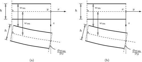
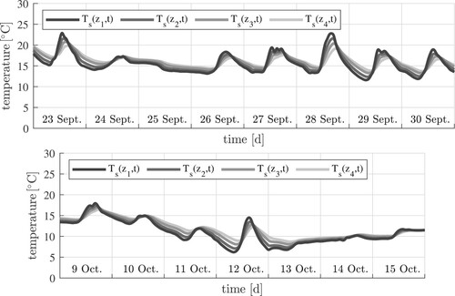
Figure A2. Temperatures measured $5\mathrm{cm}$, $9\mathrm{cm}$, $14\mathrm{cm}$ and $19\mathrm{cm}$ underneath the top surface.

Wang H., et al., 2019a. Concrete pavements subjected to hail showers: A semi-analytical thermoelastic multiscale analysis. Engineering Structures, 200, 109677.

 Web of Science ®Google Scholar

Time & Date, A, 2020. Wetterrückblick für Bad Vöslau, Niederösterreich, Österreich – Oktober 2015. Available from: https://www.timeanddate.de/wetter/oesterreich/bad-voeslau/rueckblick?month=10&year=2015. [Accessed 1 March 2022].

 Google Scholar

Mang H.A., and Hofstetter G., 2013. Festigkeitslehre. 4th ed., Springer Vieweg.

 Google Scholar