
Figures & data
Table 1. Initial values of simulation parameters and nondimensional numbers relevant to the DNS database considered for this analysis.
Table 2. The effects of Lewis number on normalized flame surface area AT/AL and normalized turbulent flame speed ST/SLwhen the statistics were extracted (i.e., t = 1.75 αT0/ ).
).
Figure 1. Distributions of on x1 − x2 mid-plane for Δ = 0.8δth (1st column), 1.6δth (2nd column), 2.8δth (3rd column) for cases A–E (1st–5th row) when the statistics were extracted (i.e., t = 1.75 αT0/
).
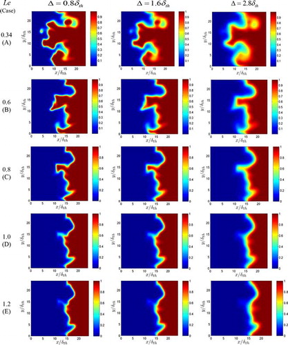
Figure 2. Variations of T1 ( —— ), T2 (![]()
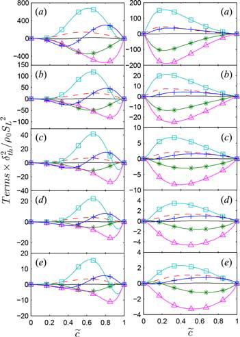
Table 3. Summary of the scaling estimates of the relevant quantities according to Gao et al. [Citation28].
Figure 3. Variations of (
![]()
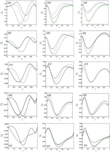
Figure 4. Variations of T2 (![]()
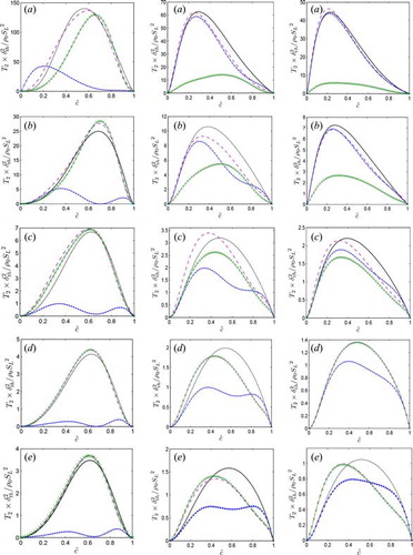
Figure 5. Variations of T3 (![]()
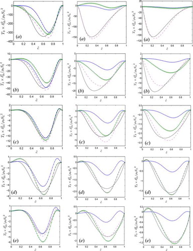
Figure 6. Variations of [T4 + f(D) − D2] (![]()
![Figure 6. Variations of [T4 + f(D) − D2] (Display full size) and [(T4)sg − (D2)sg + {f(D)}sg] (Display full size) conditionally averaged in bins of along with the predictions of Eqs. (15i) and (15ii) (Display full size) and Eq. (16) (Display full size) for Δ ≈ 0.4δth (1st column), 1.6δth (2nd column), and 2.8δth (3rd column) in cases A–E (1st–5th row). All the terms are normalized with respect to .](/cms/asset/1aaefe5a-e6b7-422d-a8c9-48fb630ccb98/unht_a_1125732_f0006_oc.jpg)