In silico prediction of dermal absorption of pesticides – an evaluation of selected models against results from in vitro testing

Figures & data

Table 1. Summary of the applied models. VE: Viable epidermis, SC: Stratum corneum, RF: Receptor fluid.

Model	Calculates	Approach	Diffusion through	Comment
Potts Guy [14]	kp	Regression	Lipid pathway	State of the art model, simple and straightforward
Mitragotri [19]	kp	Mechanistic – analytical	Tortuous lipid pathway	Equation was adapted as proposed by Lian [7] resembles that of Potts Guy
Cleek Bunge [20]	kp	Mechanistic	Lipid pathway	Corrects Potts Guy by additionally accounting for the resistance provided by the hydrophilic VE
COSMOS [21]	kp	Regression & statistical weighting	Lipid pathway
TNO [22]	% absorbed	Simplistic transition from kp to mass absorbed	n/a
Buist [23]	% absorbed in SC and RF separately	Analytical, more elaborate transition from kp to mass absorbed	n/a	Adaptable for finite doses, lag time and distribution of chemical in the stratum corneum are accounted for
IH SkinPerm [24]	% evaporated & % absorbed in SC and VE, separately	Regression – analytical	Lipid & transcellular pathway	Physical and chemical parameters such as density and vapour pressure are accounted for

Figure 1. Relation of the experimental (logExperimentalAbsorption) to the predicted absorption (logPredictedAbsorption). The experimental absorption was taken as the sum of the relative amount present in the receptor fluid, the skin sample and the tape strips – except for the first and second ones. The predicted absorption represents the absorption as calculated by each model. The diagonal line represents the function y = x.

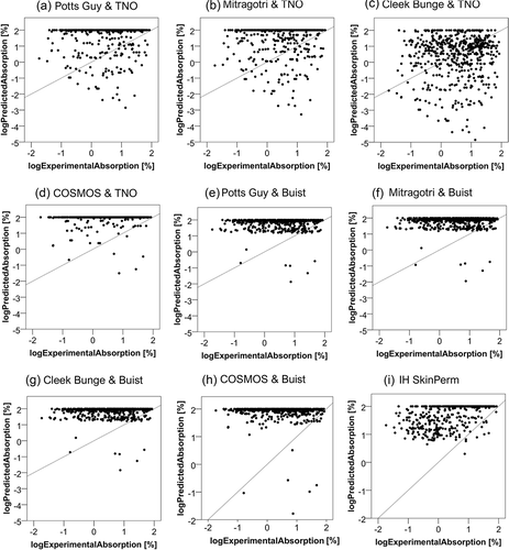
Table 2. Best performing models ranked according to the four criteria.

	Criterion 1		Criterion 2	Criterion 3		Criterion 4
	Low percentage of underestimated cases (log PF<0)		Low factor of under-estimation	High percentage of cases estimated within one order of magnitude (0≤ log PF<1)		Low percentage of highly overestimated cases (log PF≥3)
	Absolute number	Percentage	Minimum log PF	Absolute number	Percentage	Absolute number	Percentage
IH Skin Perm	11	2	−0.6	216	38	84	15
COSMOS & TNO	8	1	−2.7	187	33	145	26
COSMOS & Buist	14	2	−2.7	188	33	145	26
Potts Guy & Buist	22	4	−2.8	206	37	127	23
Cleek Bunge & Buist	21	4	−2.7	205	36	127	23
Mitragotri & Buist	27	5	−2.8	205	36	122	22
Potts Guy & TNO	64	11	−4.0	187	33	128	23
Mitragotri & TNO	75	13	−4.4	194	34	121	21
Cleek Bunge & TNO	275	49	−6.0	153	27	34	6
Total	564	100		564	100	564	100

Highlights in bold indicate best performing model(s).

Figure 2. Relation of the prediction factor to the active substance’s lipophilicity (log k_ow). Dermal absorption was predicted using the models indicated in the figure and prediction factors (PF) were calculated by dividing by experimental values. The logarithm (log PF) is plotted against measured octanol-water partition coefficients (log k_ow). In figures (a,c) open circles represent the cases out of the applicability domain. The horizontal lines mark the limit, under which the predicted is lower than the experimental absorption and the vertical the limit under which a substance is considered hydrophilic.

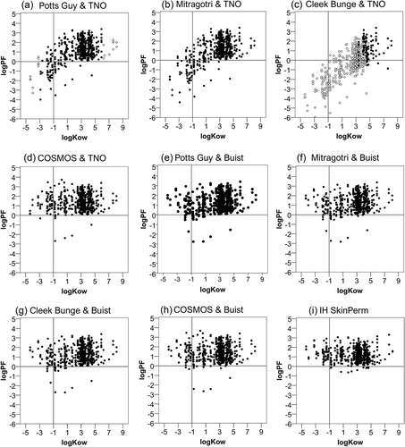
Figure 3. Relation of the prediction factor to the active substance’s molecular weight. Dermal absorption was predicted using the models indicated in the figure and prediction factors (PF) were calculated by dividing by experimental values. The logarithm (log PF) is plotted against the molecular weight. In figures (a and c) open circles represent the cases out of the applicability domain. The horizontal lines mark the limit, under which the predicted is lower than the experimental absorption.

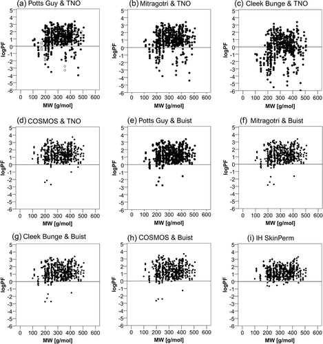
Table 3. Summary of the Pearson correlation coefficients calculated for the relationship between the log PF (log prediction factor) and lipophilicity (expressed as log k_ow) or molecular weight (MW). AD: values within applicability domain included only.

Model	Pearson correlation coefficient between log PF and log kow	p Value of the relationship between log PF and log kow	Pearson correlation coefficient between log PF and MW	p Value of the relationship between log PF and MW
Potts Guy & TNO	0.563	<0.01	0.157	<0.01
Potts Guy & TNO (AD)	0.533	<0.01	0.13	<0.01
Mitragotri & TNO	0.596	<0.01	0.131	<0.01
Cleek Bunge & TNO	0.746	<0.01	0.174	<0.01
Cleek Bunge & TNO (AD)	−0.046	0.652	−0.184	0.069
COSMOS & TNO	0.084	<0.05	0.04	0.375
Potts Guy & Buist	0.195	<0.01	0.132	<0.01
Mitragotri & Buist	0.189	<0.01	0.136	<0.01
Cleek Bunge & Buist	0.187	<0.01	0.129	<0.01
COSMOS & Buist	−0.014	0.739	0.064	0.129
IH SkinPerm	0.058	0.172	0.056	0.183

Figure 4. Distribution of the prediction factor (log PF) in different physical states. The left whisker marks the minimum value and is defined as 1.5xIQR, the left part of the box represents the 1st quartile, the middle vertical line in the box represents the median, the right part of the box represents the 3rd quartile, and the right whisker the maximum value, defined as 1.5xIQR. The circles mark the outliers and the asterisks the extremes. The vertical line in the diagram marks the limit, under which the predicted is lower than the experimental absorption. Δ marks statistically significant differences to liquids; Π to pastes, as identified by non-parametric testing performed within each model, with alpha value set to 0.05.

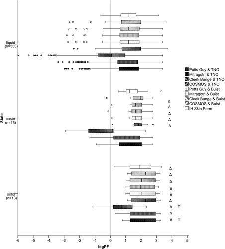
Table 4. Summary of the examined factors: expected vs. observed outcomes on the predictivity of the models.

Examined factor	Expected outcome	Observed outcome
Lipophilicity	The absorption of hydrophilic compounds may be underestimated by the models which account only for the lipophilic pathway.	For some models no effect. For some models the absorption of hydrophilic compounds is underestimated.
Molecular size	The absorption of large/small molecules may be over-/underestimated.	No effect.
Physical state	The absorption of solids may be overestimated, since most models are trained on liquids.	For all models the absorption from solids (and sometimes pastes) is overestimated to a greater extent than for liquids.
Formulation type	The absorption of dispersions, emulsions, and suspensions may be overestimated. The absorption of solutions may be overestimated only to a lesser extent.	For some models the absorption from emulsions or suspensions is overestimated to a greater extent. For some models the absorption from solutions is underestimated or overestimated to a lesser extent.
Skin thickness/type	The absorption on isolated epidermis may be underestimated.	No effect.
Irritation properties of active substance	The absorption of compounds with the potential to cause irritation may be underestimated.	For some models no effect. For some models the absorption of slight irritants was overestimated to a greater extent than non-irritants.
Occlusion after application	The absorption of compounds where the skin is occluded after application may be underestimated.	For some models no effect. For some models the absorption is overestimated to a greater extent for semi-occlusive or non-occlusive conditions compared to occlusive conditions.

Table 5. Applicability of the models as a refinement alternative to the current EFSA default values. The number of cases for which the predicted absorption would be lower than the default values as applicable according to the EFSA guidance [5] was counted. When, for those cases, predicted absorption was below experimental absorption, these were classified as refinement underestimates.

Model	Refinement of default values applicable [n out of a total of 564 cases]	Refinement underestimates [percentage]
IH SkinPerm	65	9%
COSMOS & TNO	32	22%
Mitragotri & Buist	106	23%
Cleek Bunge & Buist	86	24%
Potts Guy & Buist	88	25%
COSMOS & Buist	42	26%
Mitragotri & TNO	139	52%
Cleek Bunge & TNO	433	60%
Potts Guy & TNO	101	61%

Highlights in bold indicate models most suitable for refinement (Cleek Bunge & TNO) and with the lowest percentage of refinement underestimates (IH SkinPerm).

R.O. Potts and R.H. Guy, Predicting skin permeability, Pharm. Res. 9 (1992), pp. 663–669. doi:10.1023/A:1015810312465.

 PubMed Web of Science ®Google Scholar

S. Mitragotri, Modeling skin permeability to hydrophilic and hydrophobic solutes based on four permeation pathways, J. Control Release 86 (2003), pp. 69–92. doi:10.1016/S0168-3659(02)00321-8.

 PubMed Web of Science ®Google Scholar

G. Lian, L. Chen, and L. Han, An evaluation of mathematical models for predicting skin permeability, J. Pharm. Sci. 97 (2008), pp. 584–598. doi:10.1002/jps.21074.

 PubMed Web of Science ®Google Scholar

R.L. Cleek and A.L. Bunge, A new method for estimating dermal absorption from chemical exposure: 2. Effect of molecular weight and octanol-water partitioning, Pharm. Res. 12 (1995), pp. 88–95. doi:10.1023/A:1016242821610.

 PubMed Web of Science ®Google Scholar

P. Alov, M.T.D. Cronin, A. Diukendjieva, J.C. Madden, I. Pajeva, F.P. Steinmetz, I. Tsakovska, and C. Yang, In silico models for skin permeability and gastrointestinal absorption to facilitate extrapolation between oral and dermal administrations for repeated dose toxicity, SEURAT-1 5th Annual Meeting, Barcelona, Spain, 2015.

 Google Scholar

C. de Heer, A. Wilschut, H. Stevenson, and B.C. Hakkert, Guidance document on the estimation of dermal absorption according to a tiered approach: An update, TNO Report (1999)

 Google Scholar

H.E. Buist, J.A. van Burgsteden, A.P. Freidig, W.J. Maas, and J.J. van de Sandt, New in vitro dermal absorption database and the prediction of dermal absorption under finite conditions for risk assessment purposes, Regul. Toxicol. Pharmacol. 57 (2010), pp. 200–209. doi:10.1016/j.yrtph.2010.02.008.

 PubMed Web of Science ®Google Scholar

R. Tibaldi, W. Ten Berge, and D. Drolet, Dermal absorption of chemicals: Estimation by IH SkinPerm, J. Occup. Environ. Hyg. 11 (2014), pp. 19–31. doi:10.1080/15459624.2013.831983.

 PubMed Web of Science ®Google Scholar

European Food Safety Authority (EFSA), H. Buist, P. Craig, I. Dewhurst, S.H. Bennekou, C. Kneuer, K. Machera, C. Pieper, D.C. Marques, G. Guillot, F. Ruffo, and A. Chiusolo, Guidance on dermal absorption, EFSA J. 15 (2017), pp. 4873. doi:10.2903/j.efsa.2017.4873.

 Web of Science ®Google Scholar