Relating Latent Change Score and Continuous Time Models

Figures & data

FIGURE 1 Univariate latent change score model for two time points. The model is just identified, thus there are five free parameters: The mean ${\mu }_{\eta \left(t_0\right)}$ and variance ${\sigma }_{\eta \left(t_0\right)}^2$ of the variable at the initial time point, the mean ${\mu }_{\mathrm{\Delta }\eta \left(t_1\right)}$ and variance ${\sigma }_{\mathrm{\Delta }\eta \left(t_1\right)}^2$ of the latent change variable, and the covariance ${\sigma }_{\eta ,\mathrm{\Delta }\eta }^2$ between the two. The measurement error variances are constrained to zero. Regression paths of error terms are fixed to 1.

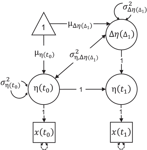
FIGURE 2 Univariate dual change score model. The dots to the right of the figure indicate that the time series can continue to any arbitrary number of time points T. No measurement took place at $t_1$ (indicated by the dashed part, which is not part of the model), thus the latent variable $\eta \left(t_1\right)$ is a phantom variable. Regression paths of error terms are fixed to 1.

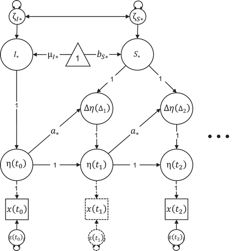
TABLE 1 Latent Change Score and Continuous Time Constraints for Time Interval ${\mathrm{\Delta }}_{j,i}$

Parameter	Latent Change Score Model	Continuous Time Model
$\mathbf{A}\left({\mathbf{\Delta }}_{j,i}\right)$	$=\left({\mathbf{A}}_{\ast }\cdot {\mathrm{\Delta }}_{j,i}+\mathbf{I}\right)$	$={\mathrm{e}}^{\mathbf{A}\cdot {\mathrm{\Delta }}_{j,i}}$
${\mathbf{S}}_i\left({\mathbf{\Delta }}_{j,i}\right)$	$={\mathrm{\Delta }}_{j,i}\cdot {\mathbf{S}}_{\ast i},$	$={\mathbf{A}}^{-1}\left[{\mathrm{e}}^{\mathbf{A}\cdot {\mathrm{\Delta }}_{j,i}}-\mathbf{I}\right]{\mathbf{S}}_i$
${\zeta }_i\left({\mathbf{\Delta }}_{j,i}\right)$	$={\zeta }_{\ast i}$	$={\int }_{t_0}^{t_{j,i}}{\mathrm{e}}^{\mathbf{A}\cdot \left(t_{j,i}-s\right)}\mathbf{G}\mathrm{d}{\mathbf{W}}_i\left(s\right)$

FIGURE 3 Univariate latent change score model. The dots to the right of the figure indicate that the time series can continue to any arbitrary number of time points T. The different types of circles indicate parameter constraints. The constraints are defined below the figure for the approximate and exact approach. For ${\mathrm{\Delta }}_j$ = 1, the model resulting from implementing the approximate parameter constraints is identical to the (LCS) model in Figure 2. Regression paths of error terms are fixed to 1.

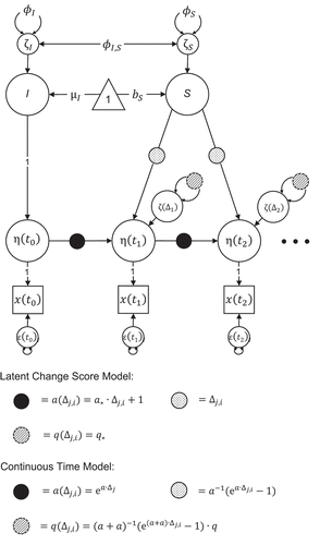
TABLE 2 Example 1: Univariate Model With Equal Time Intervals (${\mathrm{\Delta }}_{j,i}$ = 1 for all j and i)

Parameter	M1: Latent Change Score Model	M2: Latent Change Score Model Reformulated as an Autoregressive and Cross-Lagged Panel Model	M3: Continuous Time Model
Initial mean (${\mu }_I$)	1.99 (0.06)	1.99 (0.06)	1.99 (0.06)
Proportion ($a_{\ast }$) auto-effect ($a$)	−0.34 (0.01)	−0.34 (0.01)	−0.41 (0.01)
Autoregression $a\left({\mathrm{\Delta }}_{j,i}=1\right)$	0.66	0.66	0.66
Dynamic error variance ($q_{\ast }$) diffusion coefficient ($q$)	0.68 (0.01)	0.68 (0.01)	1.00 (0.01)
Dynamic error variance $q\left({\mathrm{\Delta }}_{j,i}=1\right)$	0.68	0.68	0.68
Initial variance (${\varphi }_I$)	1.99 (0.13)	1.99 (0.13)	1.98 (0.13)
−2LogL	13985.79	13985.79	13985.79
Number of free parameters	4	4	4

Note. Standard errors in parentheses. The first column (M1) contains the parameter estimates of the proportional change score model using the standard formulation by means of latent variables (Equations 3 and 5). The second column (M2) shows the reformulation of the proportional change score model as an autoregressive and cross-lagged model (Equation 7). The third column (M3) contains the parameter estimates of the continuous time model (Equation 8). The italicized parameters are obtained via the constraints in Table 1. Mplus (Muthén & Muthén, 1998–2012) was used to estimate the first two models and OpenMx (Boker et al., 2011) was used to estimate the continuous time model.

TABLE 3 Example 2: Univariate Model With Unequal Time Intervals (${\mathrm{\Delta }}_{j,i}$ = 1, 2, 3, 1, 4, 2, 3, 1, 2, 1 for j = 1, …, 10 and all i)

Parameter	M1: Latent Change Score Model Without Accounting for Unequal ${\mathrm{\Delta }}_{j,i}$	M2: Latent Change Score Model With Phantom Variables	M3: Latent Change Score Model With Phantom Variables Reformulated as an Autoregressive and Cross-Lagged Panel Model	M4: Latent Change Score Model Reformulated as an Autoregressive and Cross-Lagged Panel Model Using Definition Variables to Account for ${\mathrm{\Delta }}_{j,i}$	M5: Continuous Time Model
Initial mean (${\mu }_I$)	1.96 (0.06)	1.96 (0.06)	1.96 (0.06)	1.96 (0.06)	1.96 (0.06)
Proportion ($a_{\ast }$) auto-effect ($a$)	−0.46 (0.01)	−0.31 (0.01)	−0.31 (0.01)	−0.24 (0.01)	−0.37 (0.01)
Autoregression $a\left({\mathrm{\Delta }}_{j,i}=1\right)$	—	0.69	0.69	0.76	0.69
Dynamic error variance ($q_{\ast }$) Diffusion coefficient ($q$)	0.97 (0.02)	0.67 (0.01)	0.67 (0.01)	0.92 (0.02)	0.95 (0.01)
Dynamic error variance $q\left({\mathrm{\Delta }}_{j,i}=1\right)$	—	0.67	0.67	0.92	0.67
Initial variance (${\varphi }_I$)	1.98 (0.13)	1.98 (0.13)	1.98 (0.13)	1.98 (0.13)	1.98 (0.13)
−2LogL	15792.73	15366.23	15366.23	15545.21	15366.23
Number of free parameters	4	4	4	4	4

Note. Standard errors in parentheses. The first column (M1) contains the parameter estimates of the proportional change score model (Equations 3 and 5) without accounting for unequal time intervals. Unequal time intervals are accounted for in the second column (M2) by using phantom variables. The third column (M3) shows the reformulation of the proportional change score model as an autoregressive and cross-lagged model (Equation 7) using phantom variables to account for different time intervals. The fourth column (M4) shows the reformulation of the proportional change score model as an autoregressive and cross-lagged model. Instead of phantom variables, however, unequal time intervals are accounted for by the use of definition variables. The last column (M5) contains the parameter estimates of the continuous time model (Equation 8). The italicized parameters are obtained via the constraints in Table 1. Mplus (Muthén & Muthén, 1998–2012) was used to estimate the first four models and OpenMx (Boker et al., 2011) was used to estimate the continuous time model.

TABLE 4 Example 3: Bivariate Model With Individually Varying Time Intervals (${\mathrm{\Delta }}_{j,i}$ ˜ U[1, 4] for all j and i)

Parameter	M1: Latent Change Score Model Without Accounting for Unequal ${\mathrm{\Delta }}_{j,i}$	M2: Continuous Time Model
Initial mean (${\mu }_{I_1}$)	2.08 (0.09)	2.08 (0.06)
Initial mean $\left({\mu }_{I_2}\right)$	0.96 (0.09)	0.98 (0.06)
Proportion ($a_{\ast 11}$) auto-effect ($a_{11}$)	−0.60 (0.02)	−0.40 (0.02)
Autoregression $a_{11}\left({\mathrm{\Delta }}_{j,i}=1\right)$	—	0.67
Proportion ($a_{\ast 22}$) auto-effect ($a_{22}$)	−0.71 (0.02)	−0.56 (0.03)
Autoregression $a_{22}\left({\mathrm{\Delta }}_{j,i}=1\right)$	—	0.58
Coupling ($a_{\ast 12}$) cross-effect ($a_{12}$)	0.07 (0.02)	0.11 (0.02)
Cross-lagged effect $a_{12}\left({\mathrm{\Delta }}_{j,i}=1\right)$	—	0.07
Coupling ($a_{\ast 21}$) cross-effect ($a_{21}$)	0.12 (0.02)	0.17 (0.02)
Cross-lagged effect $a_{21}\left({\mathrm{\Delta }}_{j,i}=1\right)$	—	0.11
Dynamic error variance ($q_{\ast 1}$) Diffusion coefficient ($q_1$)	1.20 (0.03)	0.99 (0.01)
Dynamic error variance ($q_{\ast 2}$) Diffusion coefficient ($q_2$)	1.82 (0.05)	1.91 (0.03)
Dynamic error covariance ($q_{\ast 12}$) Diffusion coefficient ($q_{12}$)	0.78 (0.13)	0.48 (0.02)
Initial variance (${\varphi }_{I_1}$)	2.02 (0.18)	2.05 (0.13)
Initial variance (${\varphi }_{I_2}$)	1.82 (0.16)	2.01 (0.13)
Initial covariance (${\varphi }_{I_{1,2}}$)	0.83 (0.13)	0.97 (0.10)
−2LogL	17019.87	33517.82
Number of free parameters	12	12

Note. Standard errors in parentheses. The first column (M1) contains the parameter estimates of the bivariate proportional change score model (Equations 3 and 5), without accounting for unequal time intervals. The second column (M2) contains the parameter estimates of the continuous time model (Equation 8). The italicized parameters are obtained via the constraints in Table 1. Mplus (Muthén & Muthén, 1998–2012) was used to estimate the first model and OpenMx (Boker et al., 2011) was used to estimate the continuous time model.

FIGURE 4 Predicted trajectories of latent change score (LCS) models M1 and M2, and continuous time model M4 presented in Table 5. The gray lines represent the N = 111 observed trajectories of short-term memory as a function of age. Measurement occasions with phantom variables in the LCS models are represented by empty circles.

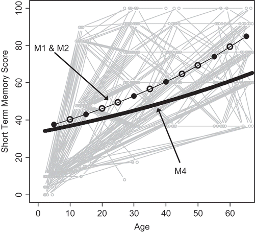
TABLE 5 Proportional Change Score Model in Discrete and Continuous Time for the Bradway–McArdle Study (M1 & M2: ${\mathrm{\Delta }}_{j,i}$ = ${\mathrm{\Delta }}_j=$ 1 for all j and i; M3: ${\mathrm{\Delta }}_{j,i}={\mathrm{\Delta }}_j=$ 2, 3, 2, 3, 2 for j = 1, …, 5 and all i; M4: ${\mathrm{\Delta }}_{j,i}$ Accounting for Individual Age of Participant)

Parameter	M1: Latent Change Score Model With Phantom Variables^a	M2: Latent Change Score Model With Phantom Variables Reformulated as an Autoregressive and Cross-Lagged Panel Model	M3: Continuous Time Model for Different ${\mathrm{\Delta }}_j$	M4: Continuous Time Model for Different ${\mathrm{\Delta }}_{j,i}$
Initial mean (${\mu }_I$)	37.67 (1.41)	37.67 (1.41)	37.67 (1.41)	34.12 (1.39)
Proportion ($a_{\ast }$) auto-effect ($a$)	0.07 (0.01)	0.07 (0.01)	0.06 (0.004)	0.01 (< 0.001)
Autoregression $a\left({\mathrm{\Delta }}_{j,i}=1\right)$	1.07	1.07	1.07	1.01
Measurement error variance (${\sigma }_{ϵ}^2$)	556.67 (41.18)	556.67 (41.18)	556.67 (41.18)	563.67 (41.06)
Initial variance (${\varphi }_I$)	21.33 (13.04)	21.33 (13.04)	21.33 (13.04)	10.64 (9.55)
−2LogL	4428.61	4428.61	4428.61	4440.70
Number of free parameters	4	4	4	4

Note. Standard errors in parentheses.

^a The first model corresponds to the proportional change score model reported by McArdle and Hamagami (2004; Table 3a, M2). Parameter estimates and model fit are identical to those reported by McArdle and Hamagami (2004).

FIGURE 5 Predicted trajectories of latent change score (LCS) models M1 and M2, and continuous time model M5 presented in Table 6. The gray lines represent the N = 111 observed trajectories of short-term memory as a function of age. Measurement occasions with phantom variables in the LCS models are represented by empty circles. To better see how the models differ in their prediction of early cognitive development, the figure in the lower right corner zooms into the part of the entire figure marked by the dashed rectangle.

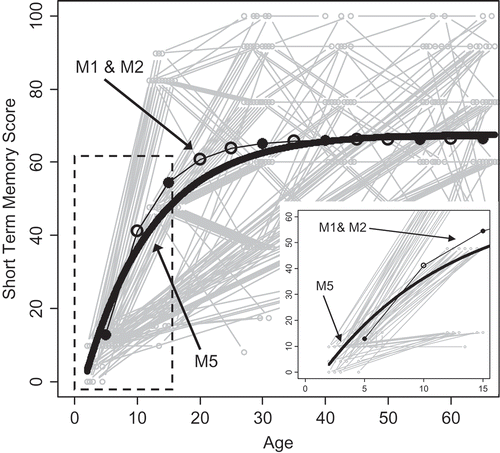
TABLE 6 Dual Change Score Model in Discrete and Continuous Time for the Bradway-McArdle Study (M1 & M2: ${\mathrm{\Delta }}_{j,i}$ = ${\mathrm{\Delta }}_j=$ 1 for all j and i; M3 & M4: ${\mathrm{\Delta }}_{j,i}={\mathrm{\Delta }}_j=$ 2, 3, 2, 3, 2 for j = 1, …, 5 and all i; M5: ${\mathrm{\Delta }}_{j,i}$ Accounting for Individual Age of Participant)

Parameter	M1: Latent Change Score Model With Phantom Variables^a, b, c	M2: Latent Change Score Model With Phantom Variables Reformulated as an Autoregressive and Cross-Lagged Panel Model^b, c	M3: Continuous Time Model for Different ${\mathrm{\Delta }}_j$^d	M4: Continuous Time Model for Different ${\mathrm{\Delta }}_j$ and Dynamic Error Instead of Measurement Error	M5: Continuous Time Model for Different ${\mathrm{\Delta }}_{j,i}$ and Dynamic Error Instead of Measurement Error
Initial mean (${\mu }_I$)	12.90 (1.35)	12.90 (1.35)	12.97	12.98 (0.60)	2.95 (1.30)
Slope mean ($b_{\ast }$) Continuous time intercept (b)	35.15 (2.00)	35.15 (2.00)	48.59	47.41 (4.29)	6.10 (0.43)
Proportion ($a_{\ast }$) auto-effect ($a$)	−0.53 (0.03)	−0.53 (0.03)	−0.72	−0.70 (0.07)	−0.09 (0.01)
Autoregression $a\left({\mathrm{\Delta }}_{j,i}=1\right)$	0.47	0.47	0.48	0.50	0.92
Measurement error variance (${\sigma }_{ϵ}^2$)	195.52 (14.52)	195.52 (14.52)	198.07	—	—
Dynamic error variance ($q_{\ast }$) diffusion coefficient ($q$)	—	—	—	408.13 (1.13)	56.47 (0.31)
Initial variance (${\varphi }_I$)	8.76 (8.12)	8.76 (8.11)	10.16	39.43 (5.29)	21.11 (7.91)
Slope variance (${\varphi }_S$) trait variance	71.69 (15.17)	71.70 (15.17)	128.61	98.97 (1.62)	1.19 (0.22)
Covariance (${\varphi }_{I,S}$)	24.81 (11.80)	24.81 (11.80)	44.41	36.79 (9.30)	−1.30 (1.53)
	[r < .99]	[r < .99]	[r < .99]	[r = .59]	[r = −0.26]
−2LogL	4066.56	4066.56	4065.22	3927.067	4034.31
Number of free parameters	7	7	7	7	7

Note. Standard errors are provided in round and correlations in squared brackets.

^a The first model corresponds to the dual change score model, reported by McArdle and Hamagami (2004; Table 3a, M4). Apart from rounding errors, parameter estimates and model fit are identical to those reported by McArdle and Hamagami (2004). ^bStandard errors might not be trustworthy due to a nonpositive definite first-order derivative product matrix. ^cCorrelation constrained to r < .99. ^dNo standard errors computed.

Muthén, L. K., & Muthén, B. O. (1998–2012). Mplus user’s guide (7th ed.). Los Angeles, CA: Muthén & Muthén.

 Google Scholar

Boker, S. M., Neale, M., Maes, H., Wilde, M., Spiegel, M., Brick, T., Spies, J., Estabrook, R., Kenny, S., Bates, T., Mehta, P., & Fox, J. (2011). OpenMx: An open source extended structural equation modeling framework. Psychometrika, 76, 306–317. doi:10.1007/S11336-010-9200-6

 PubMed Web of Science ®Google Scholar

McArdle, J. J., & Hamagami, F. (2004). Methods for dynamic change hypotheses. In K. van Montfort, J. H. L. Oud, & A. Satorra (Eds.), Recent developments on structural equation models (pp. 295–335). Dorderecht, The Netherlands: Kluwer.

 Google Scholar