
Figures & data
Table 1. Chemical composition of the brass used in the cutting path of the experimental specimens.
Table 2. The SOD and TS levels.
Table 3. The values of the machining factors used in the cutting experiments of AWJ cutting; experiment/specimen number; the SOD of 0.5–15 mm (between the cutting nozzle and the surface); the traverse speed of 5–150 mm/min; the machining time in (min, s).
Table 4. The results of the KPW readings generated by cutting specimens through the operating parameter values used in the AWJ experiments from 1 to 32, in which the KW Points are labeled 1–9 ().
Figure 1. Photograph of a water jet corporation machine.
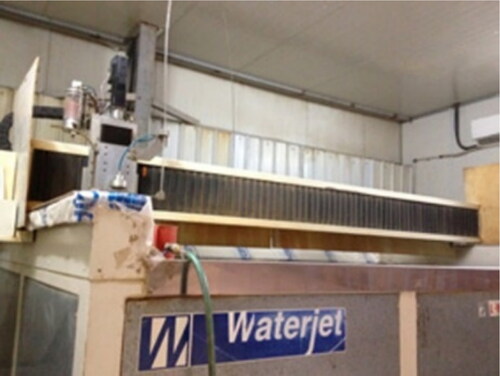
Figure 2. The cutting path design used for specimens with AWJ dimensions of 150 × 100 × 0.8 mm. The KW test Points are indicated as numbers 1–9.
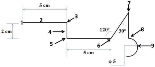
Figure 3. The magnifying device used to measure the KPW of the cut.
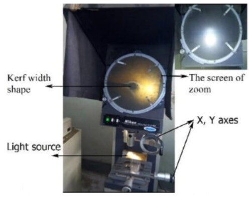
Figure 4. Illustrates the measurement device.
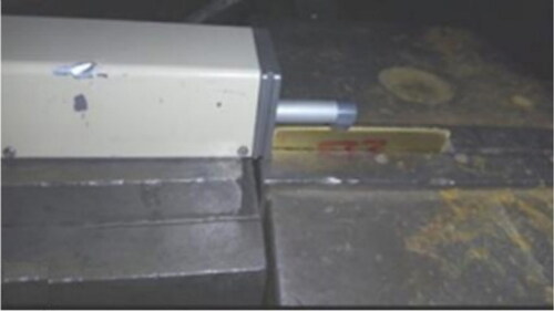
Table 5. The values of the KPW readings generated by cutting specimens using the operating parameters used in the AWJ experiments from 33 to 58, in which the KW Points are labeled 1 –9 ().
Table 6. illustrates the results of the readings of the surface roughness measurements at the edge of the cutting surface for Points 1, 2, 3 and 4 on the straight lines for all specimens from 1 to 58.
Figure 5. The KPW of (a1,a2) at 15 mm at 150 mm/min and (b1,b2) at 1 mm at 90 mm/min for Point 4.
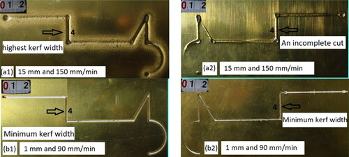
Figure 6. A comparison between the front and the back of the cutting path width of (c1, c2); (d1, d2) at 120 mm/min at 1 and 15 mm for Points 1, 2, 3, 5, 6, 7, 8 and 9.
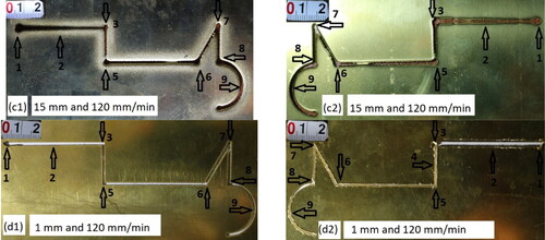
Figure 7. A comparison between the front and the back of the cutting path width of (e1, e2) and (f1, f2) at 1 mm at 5, 150 mm/min, respectively, for Point 7 and the rest of the Points.
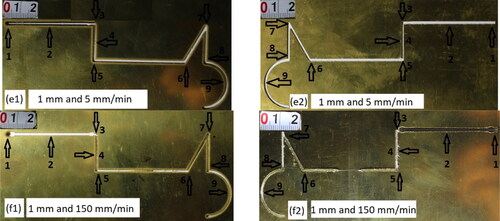
Figure 8. The front and back of the cutting path width of (g1,g2) at the minimum at 0.5 mm and 50 mm/min for Point 7.
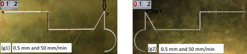
Figure 9. (a,b) KPW measurements at Points 1 –9 on the cutting path from 0.5, 1 mm, and 5 –150 mm/min for specimen numbers 1 –13: (a) 0.5 and 5, 10, 15, 20, and 50; (b) 1, 5, 10, 15, 20, 60, 90, 120, and 150.
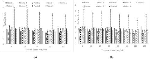
Figure 10. The locations for measuring the Ra (Points 1, 2, 3 and 4) from 0.5 to 15 mm SOD and 5 to 150 mm/min TS on a straight part of the cutting path of the backside of the specimen.
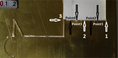
Figure 11. (a–f) Ra measurements at Points 1 –4 on the cutting path from 0.5 to 15 mm SOD and the TS from 5 to 150 mm/min on a straight line were measured as a representative for specimens numbers 1–58: (a) 0.5 mm, 5, 10, 15, 20, and 50 mm/min; (b) 1.5 mm, 5, 35, 70, 100, and 135 mm/min; (c) 2.5 mm, 5, 35, 70, 100, and 135 mm/min; (d) 3 mm, 5, 35, 70, 100, and 135 mm/min; (e) 4 mm, 5, 35, 70, 100, and 135 mm/min; (f) 5 mm, 5, 10, 20, 30, 60, 90, and 120 mm/min.
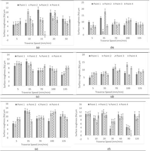
Figure 12. The cutout path back of the straight line of the specimens indicated by numbers (h2), (i2), (j2), (k2), (l2), (m2), (n2), (o2), (p2), (q2) and (r2-w2), and for the specimen (s1) from the front.
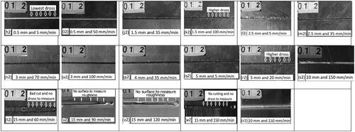
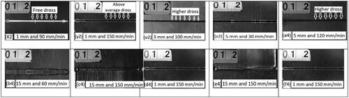
Figure 13. The cutout path back of the straight line in specimens (x2), (y2), (o2), (z2), (a4), (b4), (c4), (d4), (e4) and (f4).
Data availability statement
All the data supporting the results was provided within the article.