A shape equation for Hayward Kiwifruit

Figures & data

Figure 1. A generic ‘Hayward’ kiwifruit with the major geometrical attributes highlighted: $D_X$ = major axis; $D_Y$ = minor axis; $L$ = length

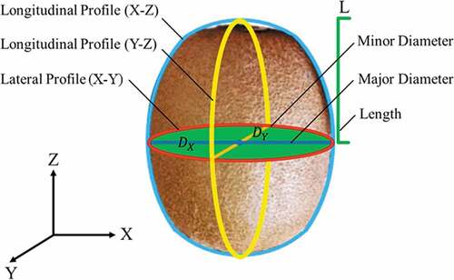
Figure 2. Empirical shape profiles in the (a) X-Z, (b) Y-Z, and (c) X-Y directions for count 36 Hayward kiwifruit. Minimum (min), average (av) and maximum (max) profiles are the result of tracing the shape of 117 fruit.^[11] Images not to scale; scale omitted to preserve data confidentiality

Figure 3. Comparison of Longitudinal Profile Functions (LPFs) with empirical shape data for Hayward kiwifruit: Red = empirical shape data; blue = new LPF (Equation 6(6) $f_2=exp\left(Z\right)-1$(6) ); and cyan = an ellipsoid

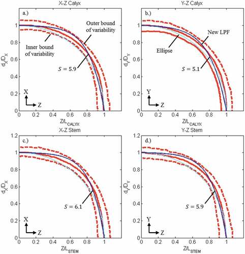
Figure 4. (a–d) Dimensionless empirical minimum, average and maximum shape profiles for count 36 Hayward kiwifruit (red) compared with the updated LPF (Equation 9(9) $d_{j,k}=\left(\left[\frac{L_k-\left(\frac{L_k}{exp\left(S\right)-1}\times \left(exp\left(\frac{S\times Z}{L_k}\right)-1\right)\right)}{2\cdot L_k}\right]+\left[\frac{\sqrt{{L_k}^2-Z^2}}{2\cdot L_k}\right]\right)\times D_j$(9) ) where $S$= 7.0 (blue; Equation (9)(9) $d_{j,k}=\left(\left[\frac{L_k-\left(\frac{L_k}{exp\left(S\right)-1}\times \left(exp\left(\frac{S\times Z}{L_k}\right)-1\right)\right)}{2\cdot L_k}\right]+\left[\frac{\sqrt{{L_k}^2-Z^2}}{2\cdot L_k}\right]\right)\times D_j$(9) ); (e) Creating a kiwifruit in COMSOL as eight parametric surfaces

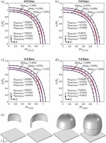
Figure 5. Numerical calculation of (a) volume and (b) surface area using the disk technique (Riddle, 1974)

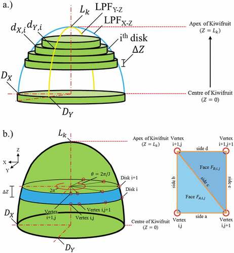
Figure 6. Efficacy of using the disk method to numerically approximate the (a) volume and (b) surface area of a sphere (radius = 1 m) as a function of the degree of numerical discretization resolution

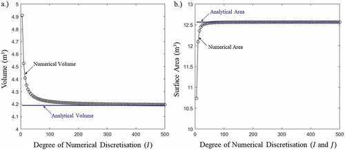
Figure 7. Comparison of predicted volumes using the new shape equation for kiwifruit (crosses; Equation 9)(9) $d_{j,k}=\left(\left[\frac{L_k-\left(\frac{L_k}{exp\left(S\right)-1}\times \left(exp\left(\frac{S\times Z}{L_k}\right)-1\right)\right)}{2\cdot L_k}\right]+\left[\frac{\sqrt{{L_k}^2-Z^2}}{2\cdot L_k}\right]\right)\times D_j$(9) and ellipsoids (circles; Equation 5)(5) $d_{j,k}=\frac{\sqrt{{L_k}^2-Z^2}}{L_k}\times D_j$(5) with measured volumes (dashed line) of kiwifruit ranging from 55.3 to 112.3 g.^[16]

Anonymous. Hayward Plots, 1997.

 Google Scholar

Riddle, D. F. Calculus and Analytic Geometry; Wadsworth Pub. Co: Belmont, CA, 1974.

 Google Scholar

Rashidi, M.; Gholami, M. Determination of Kiwifruit Volume Using Ellipsoid Approximation and Image-Processing Methods. Int. J. Agric. Biol. 2008, 10, 375–380.

 Google Scholar