Figures & data
Figure 1. Unfolded matrix.
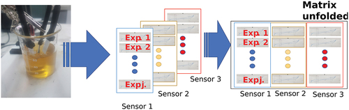
Figure 2. 3D to 2D dimensionality reduction process executed by a manifold learning method. Adapted from.[Citation51].
![Figure 2. 3D to 2D dimensionality reduction process executed by a manifold learning method. Adapted from.[Citation51].](/cms/asset/02d64571-9aa1-4cfb-9377-49aa26860df7/ljfp_a_2161571_f0002_oc.jpg)
Figure 3. K Nearest Neighbors classifier process.
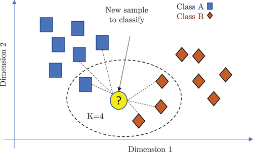
Figure 4. Leave-one-out cross-validation process.
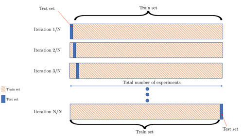
Figure 5. Experimental setup of the electronic tongue, potentiostat and electrochemical cell.
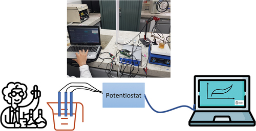
Figure 6. Voltammograms obtained in measurement with the 3 voltammetric sensors of platinum, gold, and carbon working electrodes.
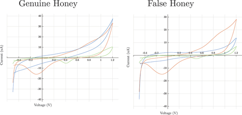
Figure 7. Pattern recognition methodology for honey classification.
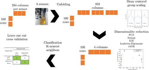
Figure 8. Unfolding signal a) before and b) after normalizing.
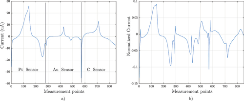
Figure 9. Classification accuracy results when applying PCA as dimensionality reduction method and after performing the LOOCV cross-validation process with the k-NN algorithm.
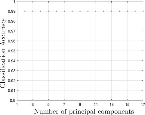
Figure 10. Two-dimensional scatter diagram of the first two principal components after executing the dimensionality reduction with the PCA algorithm.
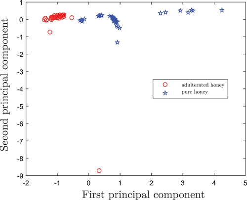
Figure 11. Classification accuracy behavior when parameter changing in each manifold learning algorithm used to perform the dimensionality reduction process. a) Graph k parameter in Laplacian Eigenmaps, b) Graph k parameter in LLE, c) Graph k parameter in Isomap and d) Perplexity p parameter in t-SNE.
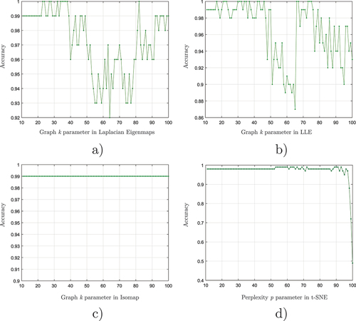
Figure 12. 2D scatter plots of the four nonlinear dimensionality reduction algorithms. a) Laplacian Eigenmaps, b) LLE, c) Isomap and d) t- SNE.
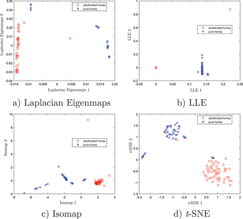
Figure 13. Accuracy behavior with a variation of the number of dimensions at the input of the k -NN classifier algorithm for a) LLE, b) t-SNE, c) Isomap and d) Laplacian Eigenmaps.
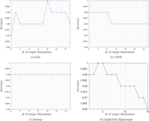
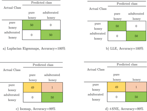
Figure 14. Confusion matrices and accuracy result of classifier k -NN evaluated with LOOCV for a) Laplacian Eigenmaps, b) LLE, c)Isomap ans d) t-SNE.