A geometric modelling approach to estimate apple fruit size by means of LiDAR 3D point clouds

Figures & data

Figure 1. a) Experimental set-up for scanning apples in indoor conditions, b) Raw point cloud of scanned apples in indoor conditions.

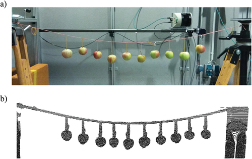
Figure 2. Randomly selected apple point cloud for each measuring date, recorded in the laboratory.

Figure 3. a) Field experimental sensor frame set-up, b) Outline of one tree with apples marked (red) and tree simulator with spheres of small (green) and large (orange) size. Heights of in-field scanned objects are marked.

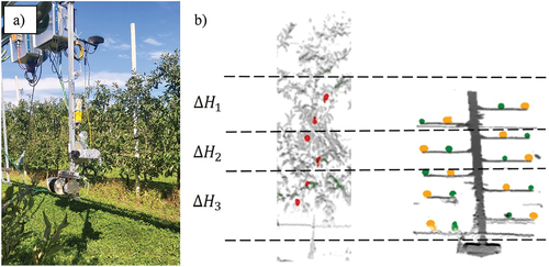
Figure 4. Diagram of an ideal sphere and its corresponding localization in Cartesian and spherical space in relation to the LiDAR position and measuring configuration.

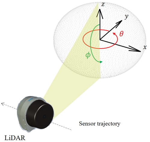
Figure 5. Flow diagram of the geometric model algorithm.

Figure 6. Fourier reference shape calculation of an example apple. a) 2D Cartesian reference point cloud, b) 1D Fourier series expansion of angular transformation of reference contour, and c) Interpolated 2D reference shape of this apple in spherical space.

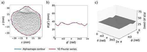
Figure 7. Eigenvector ${{\frac{n}{e}}_{\mathit{y}}}^{\mathit{fourier}}$ of the Fourier projection (blue) of a point cloud (grey) for a) random sphere of 80 mm size, and b) random apple at 151 DAFB.

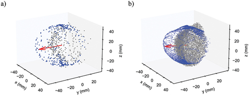
Figure 8. Diagram of a point cloud optimization results considering a randomly selected apple measured at 151 DAFB in the laboratory: a) $\mathit{RMS}{E}_{\mathit{ref}}$ curve, b) initital point cloud underestimating the curvature, c) optimal point cloud, d) increased, over-estimating error as a result of projecting the point cloud beyond its reference Fourier shape. Three marked dots in a.) are related to point cloud appearance shown in b), c) and d).

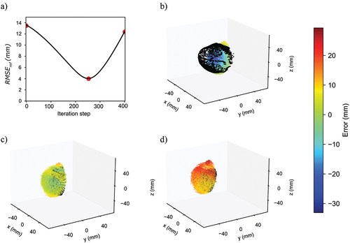
Figure 9. Computational efficiency of the geometric algorithm for the scanned spheres in laboratory (n = 6) and field conditions (n = 20), and scanned apples in laboratory (n = 60) and field conditions (n = 283).

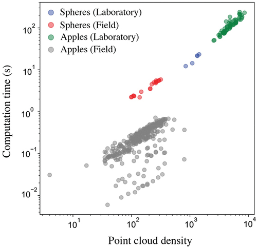
Figure 10. Optimal point cloud of indoor-measured spheres of 60 (a-c) and 80 (d-f) mm in spherical coordinates. Point clouds before approximation are shown in grey, while error is given in false colour scale.

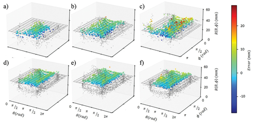
Figure 11. Optimal point cloud of spheres of 60 (a-c) and 80 (d-f) mm in Cartesian coordinates, where error is provided in false colour scale.

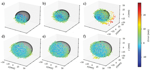
Table 1. Averaged values of root mean squared error (RMSE) and mean bias error (MBE) of point clouds measured in laboratory conditions.

	Geometric model				Mean Euclidean distance		Maximum Euclidean distance
	$\mathit{MB}{E}_{\mathit{ref}}\left(\mathit{mm}\right)$	$\mathit{RMS}{E}_{\mathit{ref}}\left(\mathit{mm}\right)$	$\mathit{MB}{E}_{\mathit{exp}}\left(\mathrm{\%}\right)$	$\mathit{RMS}{E}_{\mathit{exp}}\left(\mathrm{\%}\right)$	$\mathit{MBE}\left(\mathrm{\%}\right)$	$\mathit{RMSE}\left(\mathrm{\%}\right)$	$\mathit{MBE}\left(\mathrm{\%}\right)$	$\mathit{RMSE}\left(\mathrm{\%}\right)$
Spheres 60 mm	1.27	6.09	4.24	20.28	10.51	22.24	12.26	23.85
Spheres 80 mm	0.56	3.77	1.41	9.43	6.46	8.08	14.67	14.70
$\mathit{DAF}{B}_{60}$	−0.54	7.33	34.64	43.51	99.30	99.30	153.16	153.16
$\mathit{DAF}{B}_{74}$	−0.13	4.22	−0.07	16.21	17.45	18.75	29.48	29.48
$\mathit{DAF}{B}_{90}$	−0.91	4.67	9.94	18.73	31.22	31.22	38.74	38.74
$\mathit{DAF}{B}_{104}$	−0.55	4.75	−5.49	15.04	14.17	14.61	22.68	22.68
$\mathit{DAF}{B}_{132}$	−0.80	4.78	−9.09	13.97	4.05	5.84	8.56	8.56
$\mathit{DAF}{B}_{151}$	−0.73	4.99	−16.51	19.63	−5.07	9.83	−1.46	10.67

Figure 12. Averaged reference Fourier shapes for all monitored dates during fruit development, a) 1D Fourier shape in Cartesian coordinates, b) Interpolated 2D Fourier reference shape in spherical coordinates.

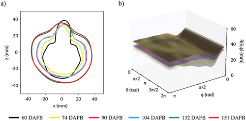
Figure 13. Performance of model approximation and error associated to the Euclidean distance calculation capturing all fruit from three canopy heights with respect to the LiDAR. Boxplots represent the point clouds before (red) and after approximation (blue). Maximum (green) and mean (blue) Euclidean distance calculations are represented by scattered points for: a) metal tree with spheres, b) 67 DAFB, c) 81 DAFB, d) 117 DAFB, e) 132 DAFB, and f) 136 DAFB.

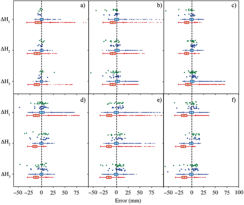
Table 2. Averaged reference values of root mean squared error ($\mathit{RMS}{E}_{\mathit{ref}}$), mean bias error ($\mathit{MB}{E}_{\mathit{ref}}$) and number of samples ($\mathit{n}$) at all vertical locations within scanned trees.

	$\mathit{n}$		$\mathit{DAF}{B}_{67}$	$\mathit{DAF}{B}_{81}$	$\mathit{DAF}{B}_{117}$	$\mathit{DAF}{B}_{132}$	$\mathit{DAF}{B}_{136}$
$\mathrm{\Delta }{H}_1$	90	$\mathit{RMS}{E}_{\mathit{ref}}\left(\mathit{mm}\right)$	7.00	7.28	4.91	6.44	6.55
		$\mathit{MB}{E}_{\mathit{ref}}\left(\mathit{mm}\right)$	3.54	2.15	−0.58	−1.23	−1.10
$\mathrm{\Delta }{H}_2$	81	$\mathit{RMS}{E}_{\mathit{ref}}\left(\mathit{mm}\right)$	8.28	5.11	5.00	7.40	5.97
		$\mathit{MB}{E}_{\mathit{ref}}\left(\mathit{mm}\right)$	1.40	−0.42	−0.48	0.30	−1.35
$\mathrm{\Delta }{H}_3$	112	$\mathit{RMS}{E}_{\mathit{ref}}\left(\mathit{mm}\right)$	7.89	5.70	8.34	7.75	7.41
		$\mathit{MB}{E}_{\mathit{ref}}\left(\mathit{mm}\right)$	0.68	−0.73	1.91	0.36	−0.48

Table 3. Field application of the geometrical model and comparison by means of $\mathit{RMS}{E}_{\mathit{exp}}$ (%) and $\mathit{MB}{E}_{\mathit{exp}}$ (%) for spheres (n = 20) and apple measuring dates (n = 283).

		Spheres	$\mathit{DAF}{B}_{67}$	$\mathit{DAF}{B}_{81}$	$\mathit{DAF}{B}_{117}$	$\mathit{DAF}{B}_{132}$	$\mathit{DAF}{B}_{136}$
Geometric model	$\mathit{RMS}{E}_{\mathit{exp}}\left(\mathrm{\%}\right)$	15.06	33.18	15.50	19.44	17.69	14.55
	$\mathit{MBE}\left(\mathrm{\%}\right)$	6.4·10^−3	33.00	14.24	18.94	16.94	13.24
Mean Euclidean distance	$\mathit{RMS}{E}_{\mathit{exp}}\left(\mathrm{\%}\right)$	15.05	27.84	25.23	168.60	29.57	132.81
	$\mathit{MBE}\left(\mathrm{\%}\right)$	−7.53	17.03	0.56	136.95	−10.52	95.66
Max Euclidean distance	$\mathit{RMS}{E}_{\mathit{exp}}\left(\mathrm{\%}\right)$	18.02	43.42	36.06	270.70	36.10	209.04
	$\mathit{MBE}\left(\mathrm{\%}\right)$	2.82	37.50	20.24	247.47	4.24	182.52

Figure 14. Linear regression between calculated and measured data for all growing periods and for all the studied models for: a) Laboratory and b) Field collected data.

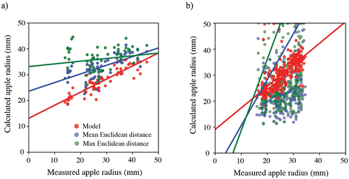
Table 4. Goodness of fit comparison between studied approaches using a linear regression for laboratory and field data.

		$R^2$	$\mathit{RMSE}\left(\mathit{mm}\right)$	$\mathit{MBE}\left(\mathit{mm}\right)$
Laboratory	Model	0.76	2.29	2.66·10^−15
	Mean Euclidean Distance	0.44	6.58	−9.47·10^−16
	Maximum Euclidean Distance	0.02	10.36	6.04·10^−15
Field	Model	0.49	4.02	1.80·10^−15
	Mean Euclidean Distance	0.21·10^−2	113.22	−4.01·10^−15
	Maximum Euclidean Distance	0.11·10^−2	192.68	3.22·10^−15