Characterization of ground-based atmospheric pollution and meteorology sampling stations during the Lake Michigan Ozone Study 2017

Figures & data

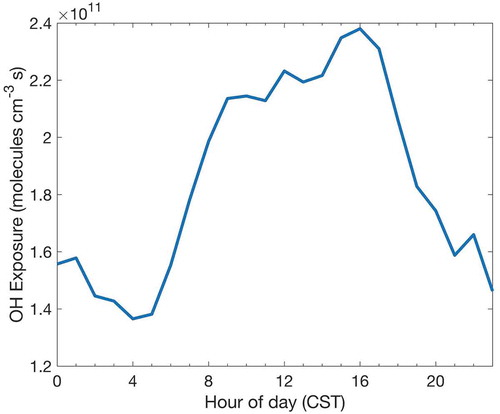
Figure 1. Overview map showing spatial coverage of LMOS 2017. Green and dark blue polygons indicate ship and aircraft operations areas, respectively. Enhanced monitoring sites at Sheboygan, WI (north) and Zion, IL (south) are mapped in more detail with insets. KUGN station is Waukegan Airport. Source: Wisconsin Department of Natural Resources (WDNR)

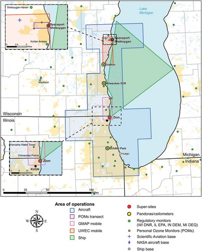
Figure 2. Maps of the EM sites for LMOS 2017 at (a) Zion IL and (b) Sheboygan WI. Also shown is Sheboygan lighthouse, used for supplemental meteorological measurements

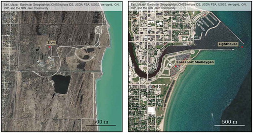
Table 1. Statistics for select measurements from Zion ground site

			Mean		Standard deviation		Median		Interquartile range		n
Variable	Time resolution	Unit	Daytime	Ozone events	Daytime	Ozone events	Daytime	Ozone events	Daytime	Ozone events	Daytime	Ozone events
N0.02–20‡	2 min	cm^-3	5711	9278	4020	4993	4717	8772	4481	7227	6844	1834
Nitric acid	1 min	pptv	839	1226	1100	995	430	876	945	1115	11319	3840
Hydrogen peroxide	1 min	pptv	2062	3432	1939	1925	1365	3400	2651	2621	11319	3840
Ammonium	12 hr	μg m^-3	0.321	0.462	0.178	0.221	0.300	0.388	0.240	0.258	32	8
Nitrate	12 hr	μg m^-3	0.129	0.156	0.152	0.120	0.086	0.120	0.081	0.078	32	8
Sulfate	12 hr	μg m^-3	0.861	1.271	0.470	0.567	0.832	1.113	0.503	0.752	32	8
PM2.5*	12 hr	μg m^-3	5.05	8.24	2.92	2.58	4.08	7.33	3.96	3.92	32	8
Ozone	1 min	ppbv	47	60	14	13	45	62	20	17	14430	3848
Air temp	1 min	C	22.3	26.7	4.3	3.1	21.3	26.5	6.2	4.3	14430	3848
Wind speed	1 min	m/s	5.00	4.42	3.28	1.99	4.60	4.20	3.20	2.70	14430	3848
Relative humidity	1 min	%	56.0	53.8	15.0	14.8	55.0	54.0	24.0	23.3	14430	3848
Nitric oxide^δ	1 min	ppbv	0.43	0.69	0.90	1.27	0.16	0.19	0.32	0.38	15360	3840
Nitrogen dioxide^δ	1 min	ppbv	1.54	3.15	2.91	4.19	0.67	1.44	1.84	2.43	15360	3840
Nitrogen oxides^δ	1 min	ppbv	1.97	3.83	3.73	5.42	0.86	1.60	1.99	2.88	15360	3840
PM2.5†	2 min	μg m^-3	6.38	10.47	4.28	3.90	5.00	9.80	6.20	6.70	7920	1920
PM10†	2 min	μg m^-3	8.27	13.68	5.66	5.33	6.70	12.70	7.80	6.90	7920	1920
Acetone	1 min	ppbv	1.38	2.02	0.54	0.37	1.17	1.96	0.81	0.45	15392	3848
Acetonitrile	1 min	ppbv	0.066	0.089	0.023	0.024	0.061	0.088	0.030	0.029	15392	3848
Benzene	1 min	ppbv	0.050	0.083	0.036	0.036	0.035	0.073	0.042	0.038	15392	3848
C4 carbonyls	1 min	ppbv	0.150	0.249	0.117	0.062	0.105	0.238	0.149	0.088	15392	3848
C5 carbonyls	1 min	ppbv	0.030	0.051	0.019	0.013	0.022	0.052	0.029	0.017	15392	3848
C6 carbonyls	1 min	ppbv	0.012	0.021	0.009	0.007	0.008	0.020	0.012	0.009	15392	3848
Isoprene	1 min	ppbv	0.698	1.56	0.805	0.830	0.351	1.53	0.917	1.06	15392	3848
Methanol	1 min	ppbv	3.99	5.76	1.76	1.58	3.49	5.74	2.04	2.77	15392	3848
Toluene	1 min	ppbv	0.068	0.107	0.087	0.092	0.039	0.071	0.053	0.077	15392	3848
Radiation	1 min	W m^-2	624	670	298	260	688	750	499	343	15500	3840
Sulfur dioxide	10 min	ppbv	0.34	0.40	0.29	0.22	0.32	0.39	0.31	0.27	1282	384

*Measured by integrated filter

†Calculated from particle size distribution

‡Particle number concentration for particles with diameters between 0.02 and 20 microns

^δNO, NO_x, and NO₂ are from the OVE (outlier values excluded) time series (see Methods).

Table 2. Statistics for select measurements from Sheboygan ground site

			Mean		Standard deviation		Median		Interquartile range		n
Variable	Time resolution	Unit	Daytime	Ozone events	Daytime	Ozone events	Daytime	Ozone events	Daytime	Ozone events	Daytime	Ozone events
Formaldehyde	1 min	ppbv	1.76	2.55	0.72	0.74	1.57	2.41	0.81	0.68	12755	1920
Formic acid	1 min	ppbv	0.628	1.161	0.505	0.638	0.530	1.040	0.530	0.750	12755	1920
Ozone	1 min	ppbv	45.5	62.8	12.7	12.6	43.6	61.7	17.3	18.6	15360	1920
Nitric oxide	1 min	ppbv	0.703	0.372	0.808	0.678	0.720	0.100	0.600	0.720	15360	1920
Nitrogen dioxide	1 min	ppbv	1.68	2.24	1.18	1.35	1.36	1.74	1.04	1.45	15360	1920
Nitrogen oxides	1 min	ppbv	2.38	2.61	1.77	1.95	2.02	1.84	1.27	2.13	15360	1920
NOy	1 min	ppbv	1.86	3.04	2.18	2.47	1.30	2.10	1.80	2.40	15360	1920
Wind speed	1 min	m/s	17.2	18.9	4.3	3.7	17.1	17.3	4.7	5.0	15360	1920
Air temp	1 min	C	64.7	66.1	15.9	12.2	66.2	68.4	26.9	18.7	15360	1920
Relative humidity	1 min	%	1.76	2.55	0.72	0.74	1.57	2.41	0.81	0.68	12755	1920

Figure 3. Wind roses of Zion (left), Waukegan (center), and Sheboygan (right) for the three cases: all hours (a, d, g), daytime hours (b, e, h) and daytime hours during ozone episodes (c, f, i). Wind speed in m/s. Zion: 1-min resolution data from May 31 to June 21. Waukegan: 1 hr resolution data from May 31 to June 21. Sheboygan: 1 min resolution data from May 21 to June 21

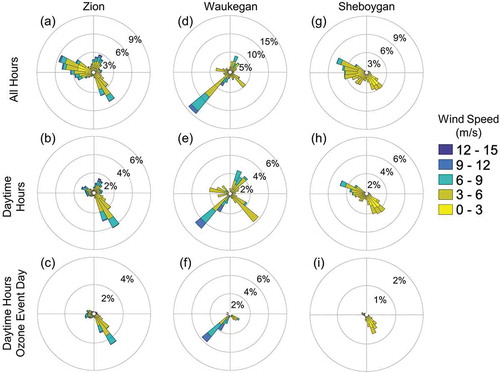
Figure 4. Spatial density plot of 48 hr back trajectory frequency for trajectories terminating at Zion, grouped by (a) daytime, (b) ozone episode daytime, (c) nighttime, and (d) all hours

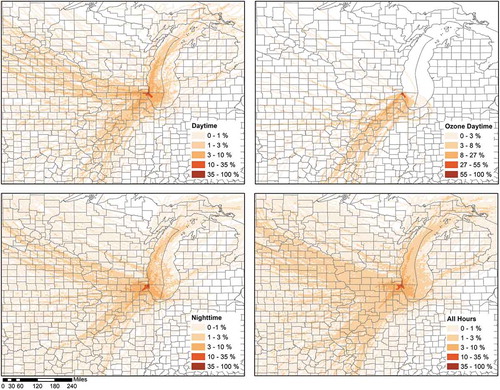
Figure 5. Spatial density plot of 48 hr back trajectories for trajectories terminating at Spaceport Sheboygan for (a) daytime, (b) ozone daytime, (c) nighttime, and (d) all hours

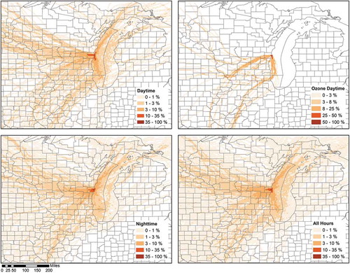
Figure 6. Pollution roses for O₃ (left) and NO_x (right) at Zion site grouped by (a, d) all hours, (b, e) daytime hours and (c, f) ozone episode daytime. Concentrations in ppb. Created using 1 min resolution data from May 31 to June 21

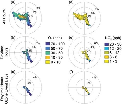
Figure 7. Pollution roses for O₃ (left) and NO_x (right) at Sheboygan site grouped by (a, d) all hours, (b, e) daytime hours and (c, f) ozone episode daytime. Concentrations in ppb. Created using 1 min resolution data from May 21 to June 21

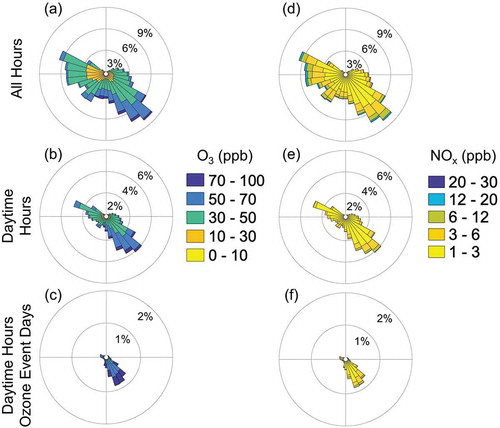
Figure 8. Cartograms centered on (a) Zion and (b) Sheboygan showing location and cumulative emissions (CO₂) of major stationary sources relative to the EM sites. Cartograms are scaled according to logarithm of distance away from the EM site

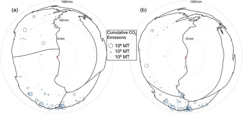
Figure 9. (a) Pleasant Prairie, (b) Zion Energy Center, (c) Waukegan Generating Station and (d) Edgewater Generating Station. Areas of circles are proportional to facility CEM cumulative CO₂ emissions and bar charts of cumulative NO_x and SO₂ emissions (MT) during LMOS 2017 from May 21 to June 21

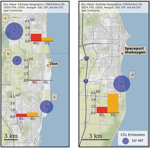
Figure 10. Results from 94 train detections over a 10 day period meeting all required criteria (meteorology and available particle size distribution measurements). The average time series is shown in panel (a) with a short pulse of audio volume indicating passage of train; particle number increases, rising from a minimum of 1930 cm^-3 to a peak of 2749 cm^-3 5.5 minutes after the train detection. Histograms of (b) particle number and (c) audio volume before and after show modest increase, and no change, respectively

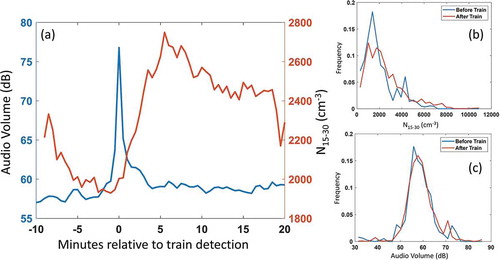
Figure 11. PMF factor time series and conditional probability functions. Abscissa units are in CST and tick marks are at midnight CST. The shading represents ozone event days

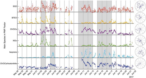
Figure 12. OH exposure (Zion, IL) boxplot for various periods of LMOS 2017. Red line is median; box encompasses 25th to 75th percentiles; whiskers terminate at median ± 1.5 IQR (interquartile range). Red crosses are outliers

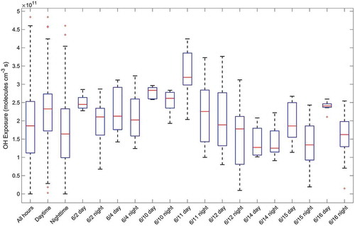
Figure 13. Diurnal pattern of OH exposure