Theoretical distinction between functional states in working memory and their corresponding neural states

Figures & data

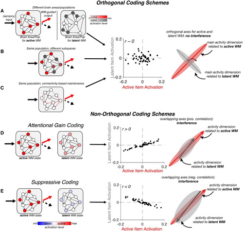
Figure 1. Summary of possible coding schemes for active vs. latent WM. Rows show different putative coding mechanisms for active versus latent WM. Left-hand column: Circuit-level depiction of various coding schemes in an example neural population. Each grey square represents a WM-coding neural population. Within the population, circles represent coding units (neurons), and arrows represent directed connections. Activated units are shown in colour (active: red, latent: grey or blue). Middle column: Correlation between activation patterns for items in an active (x-axis) or a latent (y-axis) state. Individual points indicate units. Correlations are exaggerated for illustration. Right-hand column: Neural state-space representation. When reduced to their most informative dimensions, neural patterns for active or latent items may occupy different subspaces. The extent of their overlap is a reflection of how correlated patterns are for active and latent WM. (A-C). Various coding schemes leading to orthogonal representations (no correlation between active and latent patterns). (A). Separate brain areas or separable neural populations. (B). Separate patterns in the same neural population. (C). Connectivity-based (i.e., activity-silent storage) can also separate active from latent WM by changing the weights of different connections in the population. (D-E). Non-orthogonal coding schemes. (D). Attention Gain coding separates active from latent WM through differences in amplitude, rather than different patterns. (E) Similarly, suppressive coding stores latent WM in the same neural pattern, but through a reversal of activity, leading to anti-correlated activity patterns that nevertheless occupy the same neural subspace.