On the evaluation of the takeoff time and of the peak time for innovation diffusion on assortative networks

Figures & data

Figure 1. The three panels in this figure display the increasing character of the function $k_{nn}(k)$ for networks of the three families introduced in this section. Specifically, the left panel refers to a network of the power-like family, the central panel refers to a network of the linear family, and the right panel refers to a network of the exponential family. In all cases, the maximum number $n$ of links of the network is equal to $99$, the parameter $\gamma$ (the exponent of the power-law degree distribution) is equal to $2.5$ Also, the parameters $\lambda ,\mu$ and $\nu$ are all equal to $1$.

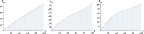
Figure 2. Log-log plots of the degree distributions obtained for networks with $n=99$ by assigning excess-degree correlations $e_{jk}=c_{\delta }/(1+j+k{)}^{\delta }$, with $\delta =2.2$, $\delta =2.4$, $\delta =2.6$ and $\delta =2.8$. The plots are ordered from the upper one ($\delta =2.2$) to the lower one ($\delta =2.8$). The degree distributions $P(k)$ behave as $c/k^{\gamma }$ with $\gamma =2.42$, $\gamma =2.61$, $\gamma =2.79$ and $\gamma =2.98$ respectively.

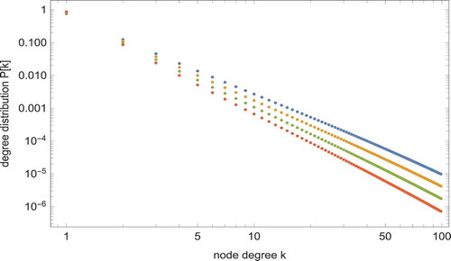
Figure 3. The two panels show the increasing character of the function $k_{nn}(k)$ for two networks with a maximum number $n$ of links equal to $99$ and excess-degree correlations as in (12) with $\delta =2.2$ (left panel) and $\delta =2.8$ (right panel).

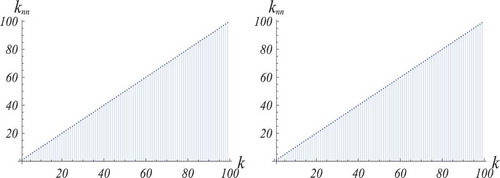
Figure 4. The left panel displays the evolution in time of the population fractions $F_j(t)$ in the case of an underlying network of the ‘power-like’ family with parameters $n=9$, $\gamma =2.9$ and $\lambda =1$. The innovation coefficient $p$ is equal to $0.03$ and the imitation coefficient $q$ is equal to $0.4$. The graphs of the functions $F_j$, as in the centre panel those of the functions $f_j$, are ordered from the upper one ($j=1$) to the lower one ($j=9$). One may observe that the largest fraction of new adopters belongs at all times to a single link class, the link class with $j=1$, which reaches its adoption peak later than the others. The fact that more connected individuals adopt earlier is a general (and rather intuitive) phenomenon. The centre panel shows the evolution in time of the nine functions $f_j(t)$, whereas the right panel displays the evolution in time of the function $f(t)$ together with that of the function $\dot{F}(t)$ relative to the original Bass equation. The values of $t$ in correspondence to which the two graphs have a maximum are the peak time of the system on the network and of the homogeneous Bass system, respectively.

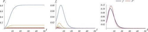
Figure 5. A portion of the graph of the function $f(t)$ of Figure 4 is here displayed with time scaling suitable to make evident the existence of an inflection point (the takeoff point) and of a maximum point (the peak point).

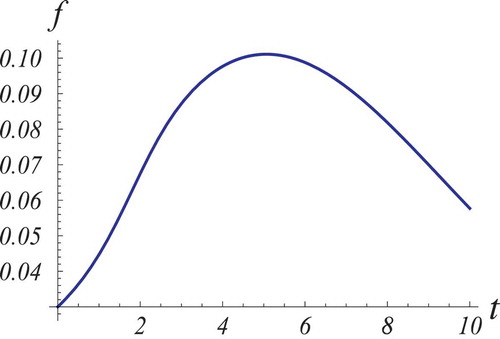
Figure 6. The panels display two surfaces, respectively, obtained through interpolation of the values of the takeoff time (left panel) and of the peak time (right panel) for the ‘power-like’ family in correspondence to the values of the parameters $\gamma$ and $\lambda$ mentioned in Table 1. Similar figures for the other two families are qualitatively similar and hence are not reported here.

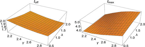
Table 1. This table provides approximate values for the takeoff time, the peak time and the assortativity coefficient of 20 networks of the ‘power-like’ family in Section 2.

‘Power-like’ family	$\lambda =0.5$	$\lambda =1.0$	$\lambda =1.5$	$\lambda =2.0$
takeoff time $t_{off}$
$\gamma =2.1$	2.049	1.934	1.843	1.783
$\gamma =2.3$	1.994	1.879	1.786	1.723
$\gamma =2.5$	1.955	1.838	1.744	1.678
$\gamma =2.7$	1.932	1.814	1.717	1.650
$\gamma =2.9$	1.925	1.807	1.708	1.638
peak time $t_{max}$
$\gamma =2.1$	3.967	3.907	3.891	3.903
$\gamma =2.3$	4.060	4.116	4.244	4.386
$\gamma =2.5$	4.277	4.454	4.655	4.816
$\gamma =2.7$	4.585	4.794	4.975	5.108
$\gamma =2.9$	4.891	5.064	5.205	5.307
assortativity coefficient $r$
$\gamma =2.1$	0.594	0.716	0.803	0.857
$\gamma =2.3$	0.626	0.734	0.811	0.861
$\gamma =2.5$	0.652	0.748	0.817	0.863
$\gamma =2.7$	0.673	0.759	0.821	0.863
$\gamma =2.9$	0.690	0.767	0.823	0.861

Table 2. This table provides approximate values for the takeoff time, the peak time and the assortativity coefficient of 20 networks of the ‘linear’ family in Section 2.

‘Linear’ family	$\mu =0.25$	$\mu =0.5$	$\mu =0.75$	$\mu =1.0$
takeoff time $t_{off}$
$\gamma =2.1$	2.136	2.113	2.075	2.017
$\gamma =2.3$	2.080	2.059	2.021	1.967
$\gamma =2.5$	2.040	2.020	1.984	1.931
$\gamma =2.7$	2.013	1.995	1.961	1.910
$\gamma =2.9$	2.002	1.985	1.955	1.905
peak time $t_{max}$
$\gamma =2.1$	4.037	4.020	3.992	3.959
$\gamma =2.3$	4.069	4.069	4.065	4.075
$\gamma =2.5$	4.200	4.219	4.248	4.302
$\gamma =2.7$	4.443	4.476	4.525	4.598
$\gamma =2.9$	4.749	4.781	4.824	4.885
assortativity coefficient $r$
$\gamma =2.1$	0.481	0.513	0.563	0.629
$\gamma =2.3$	0.530	0.555	0.598	0.654
$\gamma =2.5$	0.570	0.590	0.627	0.674
$\gamma =2.7$	0.602	0.620	0.650	0.691
$\gamma =2.9$	0.629	0.644	0.668	0.705

Table 3. This table provides approximate values for the takeoff time, the peak time and the assortativity coefficient of 20 networks of the ‘exponential’ family in Section 2.

‘Exponential’ family	$\nu =0.5$	$\nu =1.0$	$\nu =1.5$	$\nu =2.0$
takeoff time $t_{off}$
$\gamma =2.1$	2.128	2.096	2.067	2.036
$\gamma =2.3$	2.073	2.043	2.014	1.987
$\gamma =2.5$	2.033	2.006	1.976	1.949
$\gamma =2.7$	2.007	1.984	1.955	1.928
$\gamma =2.9$	1.997	1.977	1.949	1.924
peak time $t_{max}$
$\gamma =2.1$	4.032	4.008	3.989	3.970
$\gamma =2.3$	4.070	4.067	4.068	4.073
$\gamma =2.5$	4.208	4.229	4.255	4.284
$\gamma =2.7$	4.454	4.492	4.532	4.572
$\gamma =2.9$	4.758	4.791	4.827	4.861
assortativity coefficient $r$
$\gamma =2.1$	0.492	0.535	0.572	0.608
$\gamma =2.3$	0.539	0.574	0.606	0.635
$\gamma =2.5$	0.578	0.605	0.634	0.658
$\gamma =2.7$	0.609	0.631	0.656	0.677
$\gamma =2.9$	0.634	0.651	0.673	0.692

Figure 7. The cooperation network of the Top 150 companies in South Tyrol (connected part).

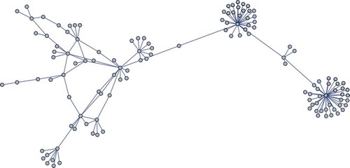
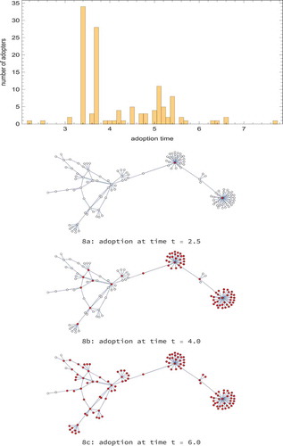
Figure 8. The top panel above shows the distribution of the peak adoption times of the nodes (companies) of the real network of Figure 7, the cooperation network of the Top 150 companies in South Tyrol, according to the Bass model in the first moment closure (Equation (13)), with parameters $q=0.35$, $p=0.03$. The adoptions in the two largest clusters are clearly visible at times 3.4 and 3.7 and those of their hubs at 2.2 and 2.4. The three panels 8a, 8b, 8c correspond to snapshots of the network at time $t=2.5$, $t=4.0$ and $t=6.0$. In each of them, the red ones in the online version (correspondent to the dark ones in the printed version) are the nodes which have adopted, whereas the white ones in the online version (light in the printed version) are the nodes which have not adopted.