The value of information about solar geoengineering and the two-sided cost of bias

Figures & data

Figure 1. Risk-Risk Trade-off. A simple illustration of the risk-risk trade-off of SG represented as a table of error types.

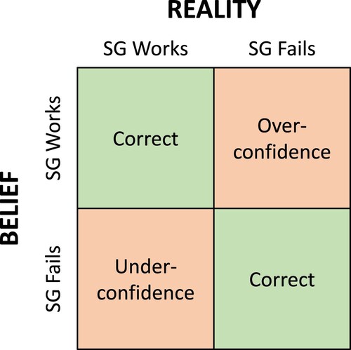
Figure 2. Model Schematic. Illustration of how SG is integrated into the extended DICE model. The left-hand side shows how the DICE damage function is augmented to include direct risks (Red) and limits to the efficacy of SG in moderating GHG-induced changes in climate (Blue). Direct risks are proportional to the amount of SG and include the costs of deployment and monitoring along with the damages directly dependent on the SG mechanism, such as ozone loss or health impacts of stratospheric aerosol. SG may moderate or exacerbate local GHG-induced climate changes. This is captured by an efficacy parameter (Blue), illustrated in the right-hand side of the figure. Regional climate responses to GHG and SG are linearized and represented as vectors in a space defined by the number of regions. The SG response vector can be decomposed into a moderating component, which exactly counteracts the effects of GHGs, and an orthogonal component which represents the imperfections in SG’s ability to restore climate changes. The angle, θ, between these linearized response vectors determines our parameterization of SG’s efficacy. Climate damages are multiplicatively scaled by the efficacy value, E, for the level of GHG-induced change in RF restored by SG, given by g. The bottom panel illustrates the efficacy of SG for different efficacy angles and levels of SG deployment. At an angle of θ = 0°, for example, SG that restores all GHG-induced RF change eliminates all climate damages; but, at an angle of θ = 45°, SG exacerbates some local climate changes and moderates others so it will only reduce aggregate climate damages by around 40%.

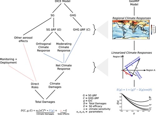
Figure 3. Value of learning about SG efficacy. (a) and (b) display the cost-benefit optimized climate instrument choices over time in the case of no learning (blue) and perfect learning in 2050 (red). Net emissions represent business-as-usual emissions net of emissions reductions and CDR. (c) and (d) display damages and carbon policy instrument costs – both mitigation and CDR costs – for no learning (blue) and perfect learning in 2050 (red). For no learning, mean damages and costs are shown. (e) displays the value of information about SG efficacy (black), ECS (orange solid), and ECS with no SG available (orange dashed). Green and pink bars show contributions to the value of information about SG efficacy from reduced climate damages (green) and reduced carbon policy costs (pink). (f) displays the expected value of partial information about SG efficacy as a function of the percent reduction in the standard deviation of priors for learning in 2030. Grey lines denote 33% and 50% reduction.

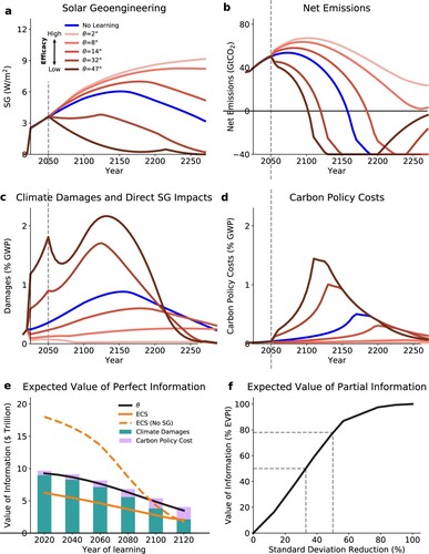
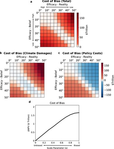
Figure 4. The cost of bias. (a), (b), and (c) show the cost of bias about SG efficacy without uncertainty. This is a quantitative version of the trade-off shown in Figure 1. Possible beliefs and realities are represented by point values. The cost of bias in SG efficacy measured by (a) reduced consumption, (b) increased climate damages, and (c) increased carbon policy costs. (d) displays the cost of bias with uncertainty. Bias is measured by parameter s which multiplicatively scales the decisionmaker’s uncertain beliefs by 1-s.

Data availability

All data generated and used in this analysis will be made publicly available upon publication.