Advancing cervical cancer diagnosis and screening with spectroscopy and machine learning

Figures & data

Figure 1. a) Cluster analysis. An overview of how the dimension reduction occurs. 1. The original matrix may have n number of columns with n variables. 2. In the example a matrix of 5 dimensions is depicted, and then exemplified that it’s not possible to plot a 5 dimension plot. 3. Depicts the step of covariance matrix creation. 4. The covariance matrix selection gives way to the eigenstuff calculation, the eigenstuff includes the eigenvectors (λ), and eigenvalues (ν), which together build the principal components. 5. Principal components now can be compared against each other, creating a 2D plot. 6. The PCs create now a reduced matrix in comparison with the input matrix, allowing an easier interpretability. b) Dendrogram of a hierarchical cluster analysis. The Dendrogram depicts where the leaves and nodes are localized. The HCA was able to find two clusters, green and red. c) K means example. The image shows where the random centroids were placed after the final iteration. The distance border, commonly Euclidean distance, helps to the data points to find the closest distance to the closest centroid.

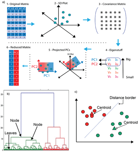
Figure 2. Overall structure of an ANN. Each ANN consists of different process units, and layers. The activation function works within each process unit.

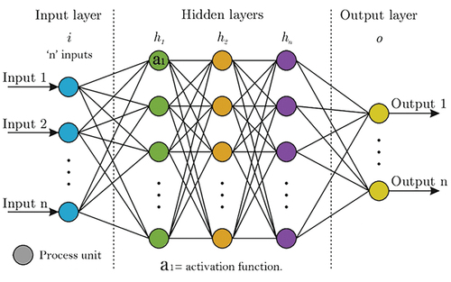
Table 1. Highlights of the supervised models presented. This table aims to provide an overall overview of advantages and disadvantages of the machine learning supervised methods.

Model	Advantages	Disadvantages
LDA	Considers the different scales and correlations between variables. LDA uses information from the features to create a new axis which in turn minimizes the variance and maximizes the class distance of the two variables.	Number of variables needs to be less than number of samples. Data must be normal distributed. Does not consider variance of each class.
PLS-DA	No need to apply PCA prior to PLS. Able to handle more descriptive variables.	Linear regression is a limitation. Number of variables needs to be less than number of samples. Does not consider variance of each class.
SVM	The algorithm works well when the class separation is clear. SVM is effective with high-dimensional spaces. Efficient when number of dimensions is greater than number of samples.	Large datasets not effective when using SVM (Large data sets definition is relative and arguably, can be bigger than 100K columns). Not performs well when classes overlap.
KNN	Easy implementation Low parameters used. Can be used for classification or regression problems. Multiclass prediction allowed.	The efficiency of the algorithm diminishes as the number of data, predictors, and variables increase.
LR	Implementation is not difficult. Easy to interpret. Allows multiclass predictions.	If the observations are less than the features the model will overfit. Linearity assumption is a limitation.
RF	Reduces data overfitting. Can be used for classification or for regression. It is not necessary to normalize data.	Requires high computational sources to create big sets of decision trees. Can take a lot of time to train the data, since it combines several decision trees.
NNs	NNs can learn by themselves. NNs can detect non-linear relationships among the data. Efficient for medical classifications.	Requires efficient and quick computational resources. The processing units can be perceived as a black box, and not being able to detect problems. Prone to overfitting.
EMs	The prediction may improve since it considers different supervised models. Predictions can be stable in bagging method. Boosting reduces bias of the model. Stacking tends to improve accuracy and keeping variance and bias low.	Interpretation can be difficult. Ensemble models can be hard to construct. Training of data can be difficult to perform.

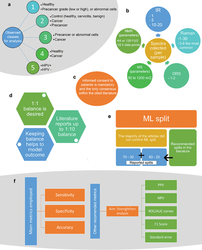
Figure 3. Method comparison found on the literature. a: Class selection. b: Spectra collection according to the spectroscopy method. c: Consent form as unique consensus. d: Reported ML balance. E: Reported ML split. F: Metrics reported and metrics recommended for ML analysis.