1,295
Views
8
CrossRef citations to date
0
Altmetric
Part A: Materials Science

Temperature dependence of effective stress in severely deformed ultralow-carbon steel

&
Pages 1979-1992 | Received 11 Dec 2015, Accepted 21 Apr 2016, Published online: 02 Jun 2016

Figures & data

Table 1. Chemical composition of the alloy used in this study.

Figure 1. Back-scattered images of the specimens with grain sizes of (a) 0.11 μm, (b) 0.43 μm, (c) 2.0 μm and (d) 9.3 μm. The specimen in (a) is the as-ARB-processed one, while those in (b)–(d) are the annealed ones.
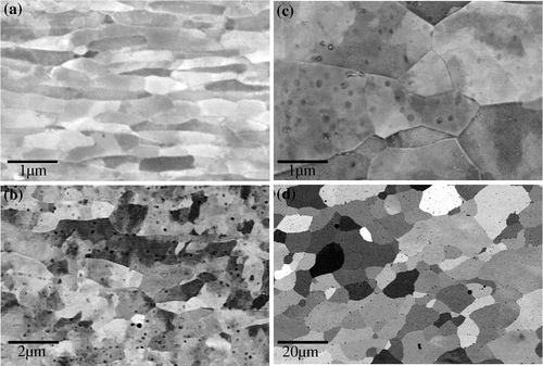
Figure 1. Back-scattered images of the specimens with grain sizes of (a) 0.11 μm, (b) 0.43 μm, (c) 2.0 μm and (d) 9.3 μm. The specimen in (a) is the as-ARB-processed one, while those in (b)–(d) are the annealed ones.

Figure 2. (colour online) Stress–strain curves for the various specimens at different temperatures, obtained using strain gages. The s–s curves are limited to the point where the strain gages became detached. The arrows indicate the points at which strain-rate jump tests were performed. (a) as-ARB-processed specimen and specimens with a grain size of (b) 0.43 μm; (c) 2.0 μm; and (d) 9.3 μm.
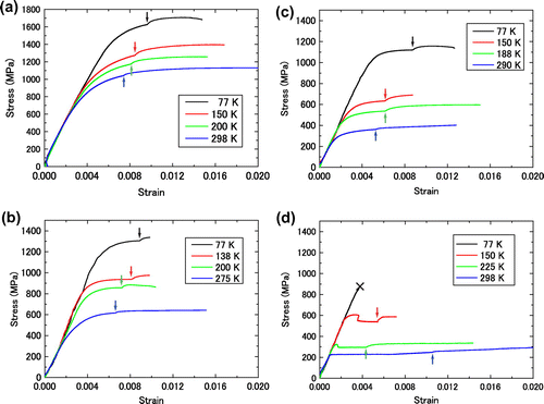
Figure 2. (colour online) Stress–strain curves for the various specimens at different temperatures, obtained using strain gages. The s–s curves are limited to the point where the strain gages became detached. The arrows indicate the points at which strain-rate jump tests were performed. (a) as-ARB-processed specimen and specimens with a grain size of (b) 0.43 μm; (c) 2.0 μm; and (d) 9.3 μm.

Figure 3. (colour online) Temperature dependence of the yield stress for the specimens with different grain sizes. The regression curves are overlaid.
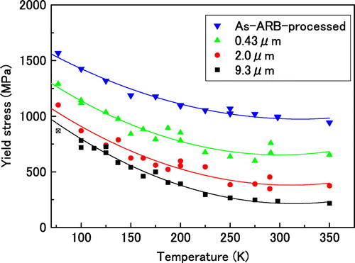
Figure 3. (colour online) Temperature dependence of the yield stress for the specimens with different grain sizes. The regression curves are overlaid.

Figure 4. SEM images of the specimen surfaces observed from the normal direction after tensile tests at room temperature ((a)–(d)) and 100 K ((e)–(h)). The tensile tests were continued until the specimens ruptured after local deformation. (a), (e) as-ARB-processed specimen and specimens with a grain size of (b), (f) 0.43 μm; (c), (g) 2.0 μm; and (d), (h) 9.3 μm.
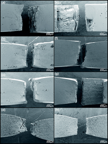
Figure 4. SEM images of the specimen surfaces observed from the normal direction after tensile tests at room temperature ((a)–(d)) and 100 K ((e)–(h)). The tensile tests were continued until the specimens ruptured after local deformation. (a), (e) as-ARB-processed specimen and specimens with a grain size of (b), (f) 0.43 μm; (c), (g) 2.0 μm; and (d), (h) 9.3 μm.

Figure 5. (colour online) Temperature dependence of the effective stress for the specimens with different grain sizes. The regression curves are overlaid.
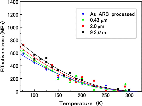
Figure 5. (colour online) Temperature dependence of the effective stress for the specimens with different grain sizes. The regression curves are overlaid.

Figure 6. (colour online) Temperature dependence of the activation volume for the specimens with different grain sizes.
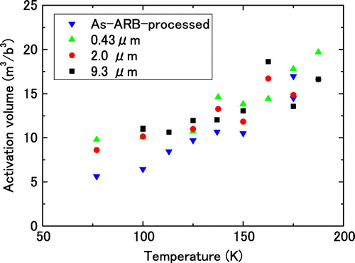
Figure 6. (colour online) Temperature dependence of the activation volume for the specimens with different grain sizes.

Figure 7. (colour online) Temperature dependence of the activation energy for dislocation gliding at temperatures lower than 200 K. The activation energy values of the as-ARB-processed specimen are lower than those of the others.
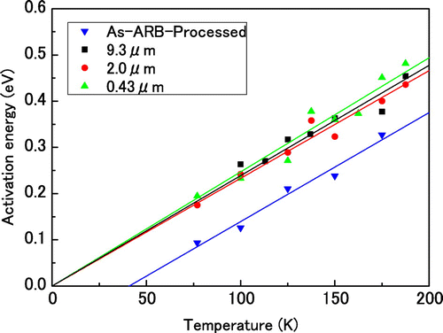
Figure 7. (colour online) Temperature dependence of the activation energy for dislocation gliding at temperatures lower than 200 K. The activation energy values of the as-ARB-processed specimen are lower than those of the others.

Figure 8. (colour online) Schematics showing the change in the activation energy for dislocation gliding with a change in the effective stress.
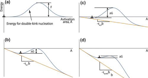
Figure 8. (colour online) Schematics showing the change in the activation energy for dislocation gliding with a change in the effective stress.

Figure 9. (colour online) Schematic drawing of energy-activation area curves, indicating the effects of long-range barriers on the thermally activated process. The period of the long-range barrier is five times than that of the short-range barrier. (a) The long-range barrier is negligible. (b) The maximum height of the long-range barrier is 0.2 times than that of the short-range barrier, which is the sum of (a) and (d). (c) The maximum height of the long-range barrier is the same as that of the short-range barrier, which is the sum of (a) and (e). (d) A long-range barrier with a low amplitude. (e) A long-range barrier with a high amplitude.
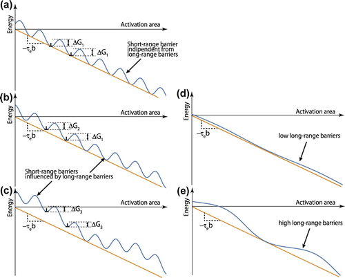
Figure 9. (colour online) Schematic drawing of energy-activation area curves, indicating the effects of long-range barriers on the thermally activated process. The period of the long-range barrier is five times than that of the short-range barrier. (a) The long-range barrier is negligible. (b) The maximum height of the long-range barrier is 0.2 times than that of the short-range barrier, which is the sum of (a) and (d). (c) The maximum height of the long-range barrier is the same as that of the short-range barrier, which is the sum of (a) and (e). (d) A long-range barrier with a low amplitude. (e) A long-range barrier with a high amplitude.