Dynamic grain models via fast heuristics for diagram representations

Figures & data

Table 1. Comparison of H1 and H2.

Performance characteristics	H1	H2
Accuracy (in %)	92.98652	92.98658
Relative cluster weight error	0.02869	0.02869
Relative centroid error (in μm)	0.64346	0.64347
Relative covariance error (in μm${}^2$)	15.25372	15.25376
Correct neighbourhoods (in %)	42.30118	42.30118
Correct neighbourhoods up to 1 Error (in %)	80.54146	80.54146
Correct neighbourhoods up to 2 Errors (in %)	94.92386	94.92386
Running time (in s)	1.49641	0.00000

Figure 1. A family of grain scans involving a parameter β to illustrate differences between H1 and H2. Top, from left to right: Grain scans for $\text{β}=0.1$, $\text{β}=0.5$, and $\text{β}=0.9$. Grain $G_1$ (orange [light gray]) fills the square $[0,\text{β}]\times [0,\text{β}]$, $G_2$ (blue [gray]) fills the rest of the unit square. The bottom row shows the computed ellipses $c_i+{\mathbb{B}}_{A_i}^2$ with $A_i=\left(\mathrm{\Sigma }\right(G_i){)}^{-1}$ for i = 1, 2.

Figure 2. Ratios ${\nu }_i/\mathrm{v}\mathrm{o}\mathrm{l}\left({\mathbb{B}}_{A_i}^2\right)$ of the areas of the grain and the corresponding ellipsoid for i = 1 (orange [light gray]) and i = 2 (blue [gray]) as a function of β.

Figure 3. Diagrams for the family of grain scans from Figure 1 obtained via H1 (top row) and H2 (bottom row).

Figure 4. Ratio of the area ${\nu }_i$ of the original grain and the area of the corresponding diagram cell obtained by H1 (left) and H2 (right) for i = 1 (orange [light gray]) and i = 2 (blue [gray]) as a function of β.

Figure 5. Accuracy (within the cross-validation paradigm) of the interpolation/extrapolation model plotted for each $t_0,\dots ,t_{14}$ using polynomials of degree 1, 2, and 3, respectively for the fit.

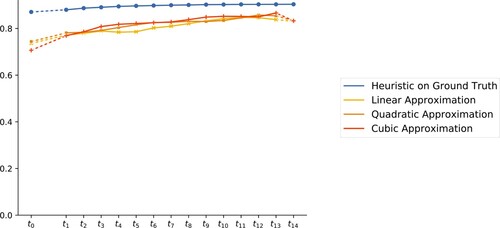
Figure 6. Visual comparison of diagrams obtained from full data (available for $t_0,\dots ,t_{14}$) and the interpolation/extrapolation model that uses all data except for the respective moment in time. A fixed 2D slice through the 3D data set at times $t_0$, $t_5$, $t_9$ and $t_{13}$ (top row); the corresponding diagram representation obtained via H1 (2nd row) and, respectively, via the interpolation/extrapolation model that uses only data from the other moments in time and best-fitting quadratic polynomials (3rd row); symmetric difference between the images from the 2nd and 3rd row (bottom row).

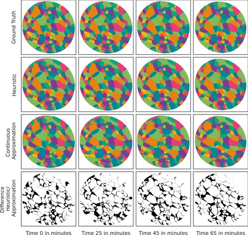
Table 2. Variance of ${\mathrm{\Gamma }}_{t_{\ell }}^{\frac{3}{2}}$ for $\ell \in \{0,1,\dots ,14\}$ of persistent grains.

	$t_{\ell +0}$	$t_{\ell +1}$	$t_{\ell +2}$	$t_{\ell +3}$	$t_{\ell +4}$
$\ell =0$	$6.409\cdot {10}^{-8}$	$6.214\cdot {10}^{-8}$	$5.130\cdot {10}^{-8}$	$3.016\cdot {10}^{-6}$	$2.544\cdot {10}^{-7}$
$\ell =5$	$6.719\cdot {10}^{-6}$	$5.839\cdot {10}^{-6}$	$1.057\cdot {10}^{-5}$	$7.025\cdot {10}^{-4}$	$9.815\cdot {10}^{-7}$
$\ell =10$	$2.286\cdot {10}^{-4}$	$7.425\cdot {10}^{-5}$	$5.749\cdot {10}^{-5}$	$1.185\cdot {10}^{-3}$	$1.823\cdot {10}^{-5}$

Table 3. Variance of ${\mathrm{\Gamma }}_{t_{\ell }}^{\frac{3}{2}}$ for $\ell \in \{0,1,\dots ,14\}$ of non-persistent grains.

	$t_{\ell +0}$	$t_{\ell +1}$	$t_{\ell +2}$	$t_{\ell +3}$	$t_{\ell +4}$
$\ell =0$	$7.570\cdot {10}^{-3}$	$1.040\cdot {10}^{-2}$	$4.915\cdot {10}^{-3}$	$1.974\cdot {10}^{-2}$	$2.993\cdot {10}^{-3}$
$\ell =5$	$1.278\cdot {10}^{-2}$	$1.834\cdot {10}^{-2}$	$2.790\cdot {10}^{-2}$	$4.158\cdot {10}^{-3}$	$8.959\cdot {10}^{-3}$
$\ell =10$	$2.608\cdot {10}^{-2}$	$2.804\cdot {10}^{-2}$	$2.955\cdot {10}^{-2}$	$3.541\cdot {10}^{-3}$	−

Table 4. Coefficients estimated by maximum likelihood estimation and their p-values for the described logistic regression model.

	Coefficient	p-value
${\text{β}}_0$ (intercept)	−4.0537	<0.0001
${\text{β}}_1$ (volume)	−0.0010	<0.0001
${\text{β}}_2$ (size parameter)	−1.0924	<0.0001