Equivalent threshold sound pressure levels for click and CE-Chirp^® stimuli delivered by the SnapPROBE™

Figures & data

Figure 1. SnapPROBE™ inserted into an infant ear and close-ups, with and without the ear tip attached. Pictures from Interacoustics A/S.

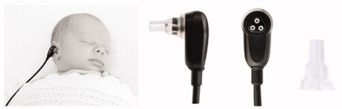
Figure 2. Frequency response of the SnapPROBE™ and an ER-3A insert earphone.

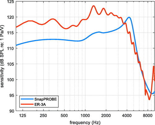
Figure 3. Pure-tone audiograms for 50 (25 left and 25 right) ears measured with a RadioEar DD45 headset. Thick line illustrates the mean.

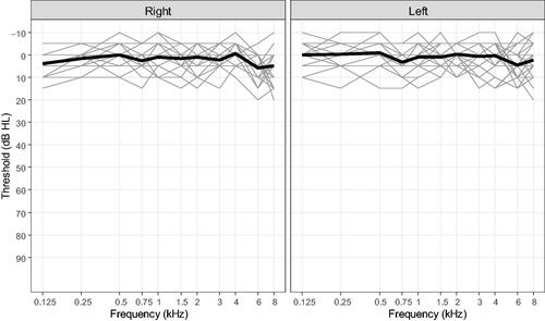
Figure 4. SnapPROBE™ ear tips modified with coloured “mushroom” parts for the purpose of fitting the infant ear tips to the adult test subjects in the study.

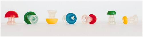
Figure 5. Illustrations based on acoustic measurements in a 711 coupler of all stimuli used, as indicated in each left-hand panel. All stimuli were scaled to produce the same spectrum level within their respective bandwidth. Left: waveforms. Right: magnitude spectrum shown for a 60-dB range.

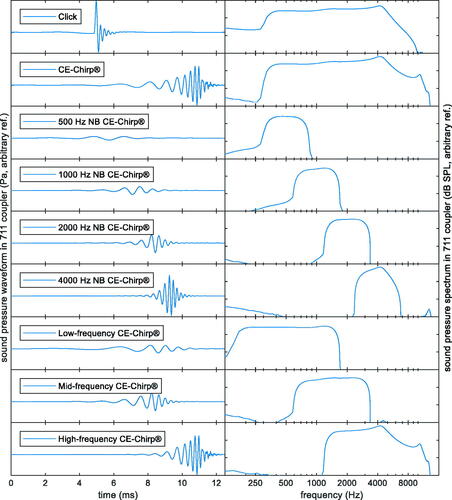
Figure 6. The ear simulator (711 coupler) (white arrow) with the SnapPROBE™ (black arrow) attached using the custom-made adaptor (black and white arrow).

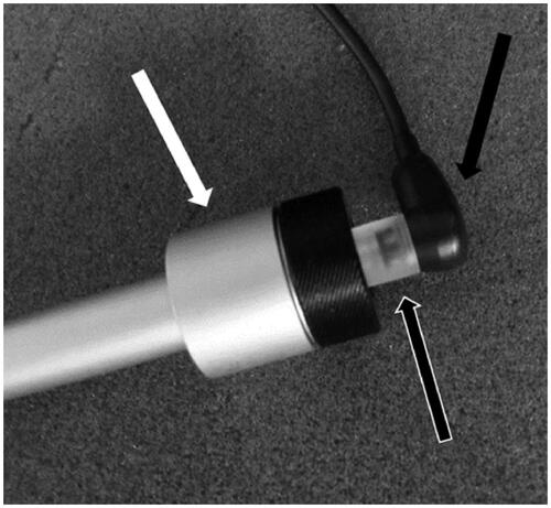
Figure 7. Example of sound-pressure waveform (blue line) of a stimulus train, with individually determined maximum and minimum peak sound pressures (bold red lines). The example is the Low-frequency CE-Chirp®.

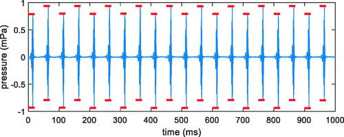
Table 1. ETSPL values for the specified stimuli presented through the SnapPROBE™, in terms of p-p.e.SPL and RMS signal levels and compared to ETSPL values (in terms of p-p.e.SPL) among different probes.

Stimulus	SnapPROBE™ RMS signal level (20/s)	SnapPROBE™ p-p.e.SPL	Titan IOW probe p-p.e.SPL	ER-3A insert earphone p-p.e.SPL
Click	16.1 dB	37.4 dB	33.5 dB	35.5 dB
CE-Chirp®	17.0 dB	34.1 dB	32.0 dB	31.5 dB
NB500 CE-Chirp®	17.3 dB	29.8 dB	N/A	25.5 dB
NB1000 CE-Chirp®	14.6 dB	30.1 dB	N/A	24.0 dB
NB2000 CE-Chirp®	18.1 dB	36.1 dB	N/A	30.5 dB
NB4000 CE-Chirp®	13.7 dB	32.9 dB	N/A	34.5 dB
Low-frequency CE-Chirp®	16.9 dB	29.7 dB	27.5 dB	N/A
Mid-frequency CE-Chirp®	15.3 dB	31.4 dB	N/A	N/A
High-frequency CE-Chirp®	16.2 dB	33.9 dB	32.0 dB	N/A

ER-3A values were compiled by Elberling and Esmann (2017); Titan IOW values are from Interacoustics A/S (2020, p. 98). As the Mid-frequency CE-Chirp® was created for this study there is no other study available for comparison.

Elberling, C., and L. C. Esmann. 2017. “Calibration of Brief Stimuli for the Recording of Evoked Responses from the Human Auditory Pathway.” The Journal of the Acoustical Society of America 141 (1): 466–474. doi:https://doi.org/10.1121/1.4974145.

 PubMed Web of Science ®Google Scholar

Interacoustics A/S. 2020. Instructions for use Titan. www.interacoustics.com/tympanometry/clinical-diagnostic/titan

 Google Scholar