Evaluating schematic route maps in wayfinding tasks for in-car navigation

Figures & data

Figure 1. Example of the input (non-schematized) and output (schematized) route map produced by the method described by Galvão et al. (2020)

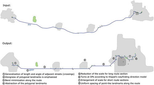
Table 1. Research questions and hypotheses

Research Questions	Hypotheses
RQ1: Do schematic route maps require less physical interaction (pan and zooming actions)?	H1.1: Schematic route maps require fewer zoom interactions.
	H1.2: Schematic route maps require less panning interactions.
RQ2: Do schematic route maps extend the visibility of the route’s surroundings?	H2: Schematic route maps result in landmarks being visible on the screen for longer.
RQ3: Do schematic route maps result in better memorability of the environment depicted on the map?	H3.1: Schematic route maps result in a significantly higher chance for recalling landmarks.
	H3.2: Schematic route maps result in a topologically more accurate recall of global landmarks.
RQ4: Are schematic route maps suitable for driving, i.e. do they (or do they not) negatively affect driving performance?	H4: Schematic route maps do not increase the number of wrong turns during map-supported driving.

Table 2. Experimental tasks and main variables measured to test our hypotheses

Research Questions	Hypotheses	Tasks	Measured variables
RQ1	H1.1	RIO & Driving	Number of zoom interactions.
	H1.2	RIO & Driving	Total length of panning (cm).
RQ2	H2	RIO & Driving	Time each landmark was visible (s).^a
RQ3	H3.1	RIO & Driving	Number of recalled landmarks.^b
	H3.2	RIO & Driving	Landmark placement topological accuracy.^b
RQ4	H4	Driving	Number of wrong turns.

^aZooming and panning actions may cause some landmarks to move out of the map’s viewport. ^bMeasures obtained from a memory test conducted after the wayfinding tasks.

Figure 2. Route 1 a) non-schematic vs b) schematic map type at initialization (lowest zoom level). Maps size was constantly 150 × 75 mm during the experiment. Label overlaps disappeared when participants zoomed in

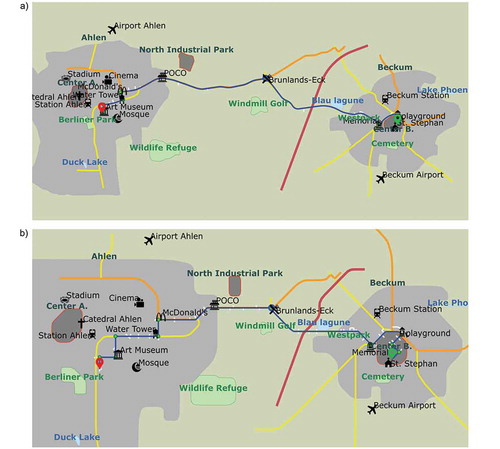
Figure 3. Route 2 a) non-schematic vs b) schematic map type at initialization (lowest zoom level). Maps size was constantly 75 × 150 mm during the experiment. Label overlaps disappeared when participants zoomed in

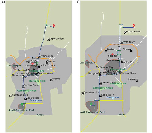
Figure 4. Route instruction ordering (RIO) web application interface. On the left, the interactive route map, on the right, the sortable list of instructions

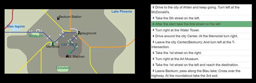
Figure 5. Situated route reading task implemented in the virtual-reality driving simulator: a) 3D city model created with CityEngine and SketchUp (here showing part of Route 2 from above). b) Hardware setup. c) A user navigating in the virtual environment while using the interactive map application on the tablet

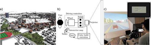
Figure 6. Examples of typical map view during the driving task: a) Route 1 type non-schematic (on the left) vs. b) Route 1 type schematic. The map dimension is fixed (150x75 mm) but participants can zoom and pan to a desired focus point. The maps are always north-oriented and rotations are not allowed. The yellow car icon indicates the driver’s virtual location on the route

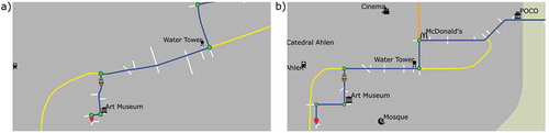
Figure 7. The landmark placement application interface for Route 1 type schematic. Only the landmarks recalled previously in the landmark recall test can be placed on the base map. For polygonal landmarks, the user first needed to drag and drop the landmark’s bounding box onto the desired position before seeing the polygon’s true shape

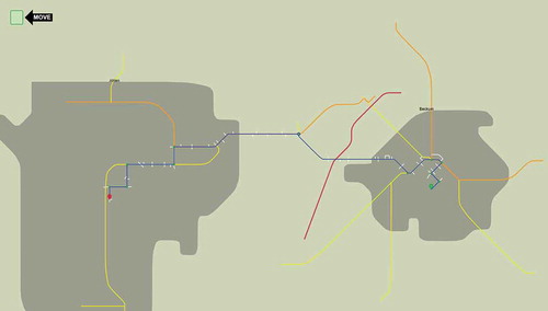
Table 3. Differences between the RIO task and the driving task: prospective vs. situated route reading

	RIO	Driving
Procedure	-Ordering textual instructions according to the presented route map. -Map interaction with the mouse. -No time pressure.	-Driving in a virtual environment following a route map. -Map interaction with the touch-screen. -Indirectly imposed time pressure (the goal was to reach the destination quickly, and the map was only viewed when stopped).
Communicating spatial information	-The map and the instructions are always visible.	-The map is only visible on request (requires stopping the vehicle).
	-Own position not relevant.	-Own position visualized with a car icon.
	-Environment surrounding the user not applicable.	-Environment surrounding the user always visible on the projector screen from the egocentric perspective.
	-Some landmarks are mentioned in the text.	-Some landmarks are visible from the route.
Cognitive processes involved	-Understanding textual instruction is necessary.	-No textual instructions.
	-Matching the map with textual instructions.	-Matching the map with the virtual environment.
	-Does not require taking navigational actions (e.g. turning).	-Requires taking navigational actions.
	-No memorization required.	-Requires memorization.
Measured variables	-Map use time is equivalent to the duration of the entire task.	-Map use time is lower than the duration of the entire driving task.
	-Performance errors not measured.	-Performance errors measured in the form of wrong turns.

Figure 8. Experimental design and procedure. The experiment is composed of two tasks (RIO and driving) and two memory tests: a landmark recall and a landmark placement test. In this process diagram, the letter ”A” and ”B” is used to indicate two different routes, directions, or map types. For example, if ROUTE_A is the Route 1, then ROUTE_B is the Route 2; and if ROUTE_A is the Route 2, then ROUTE_B is the Route 1

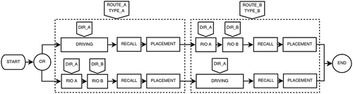
Table 4. Descriptive map interaction statistics: mean (standard deviation)

Task	Map type	Zoom^b	Pan in cm	Time in sec.
RIO^a	Non-schematic	168.33 (92.84)	313.02 (151.84)	564.86 (225.03)
	Schematic	50.46 (39.98)	177.22 (95.11)	519.89 (211.89)
Driving	Non-schematic	13.77 (8.19)	81.32 (57.94)	174.46 (102.45)
	Schematic	5.73 (5.20)	24.76 (20.97)	148.91 (71.82)

^aAggregated data for both directions. ^bAggregated counts of zoom-in and zoom-out interactions.

Table 5. Descriptive statistics of landmarks’ visibility, correct recall, and correct placement: mean (standard deviation)

Task	Map type	Visible in %	Recall in %	Placement^b in %
RIO^a	Non-schematic	24.96(19.63)	41.92(49.37)	31.62(47.10)
	Schematic	36.85(25.86)	44.56(49.74)	62.79(48.91)
Driving	Non-schematic	25.11(17.80)	35.80(47.97)	35.56(48.40)
	Schematic	51.88(31.30)	39.27(48.87)	54.90(50.25)

^aAggregated data for both directions. ^bConsidering only global landmarks.

Figure 9. Recall of landmarks: a) After the RIO task, 44.6% of the map’s point-like landmarks were recalled by non-schematic map type users, while 48.9% by the schematic map type users. For polygonal landmarks, 36.6% by non-schematic users and 35.9% by schematic users. b) After the driving task, 43.4% of the map’s point-like landmarks were recalled by non-schematic map type users, while 50.9% by the schematic map type users. For polygonal landmarks, 20.4% by non-schematic users and 15.9% by schematic users. c) After the driving task, 7.1% of the point-like and 8.4% of the polygonal foils were (erroneously) recalled. After the RIO task, 4.9% of the point-like and 7.2% of the polygonal foils were (erroneously) recalled

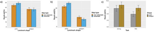
Figure 10. Topological subdivisions are formed by the street network and the city’s boundaries. a) Route 1 and b) Route 2

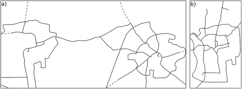
Figure 11. Topologically correct placement: Percentage of the correctly recalled global landmarks that were placed in the correct topological region, aggregated by the map type. Excluding responses for which participants reported 0% of confidence

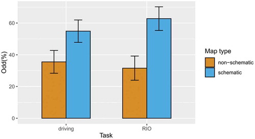
Table 6. Confirmation of hypotheses summary

Hypotheses	Description	Task	Status
H1.1	Schematic route maps require fewer zoom interactions.	RIO	Confirmed
		Driving	Confirmed
H1.2	Schematic route maps require less panning interaction.	RIO	Confirmed
		Driving	Confirmed
H2	Schematic route maps result in landmarks being visible on the screen for longer.	RIO	Confirmed
		Driving	Confirmed
H3.1	Schematic route maps result in a more significant chance of recalling landmarks.	RIO	Not confirmed
		Driving	Not confirmed^a
H3.2	Schematic route maps result in a topologically more accurate recall of global landmarks	RIO	Confirmed
		Driving	Not confirmed
H4	Schematic route maps do not increase the number of wrong turns during map-supported driving.	Driving	Confirmed

^aHigh probability of the positive effect for point-like landmarks.

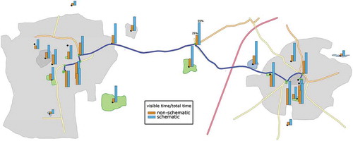
Figure 12. The difference in the landmarks’ relative visibility between non-schematic (orange) and schematic (blue) map type in the driving task for Route 1 (similar results were found for Route 2 and in the RIO task). The bars show each landmark’s mean visible time divided by the map use time, calculated as $t_i\times 100/T$. Where $T$ is map use time, and $t_i$ is the time for which the given landmark $i$ was present within the map’s viewport

Galvão, M., Krukar, J., Nöllenburg, M., & Schwering, A. (2020). Route schematization with landmarks. Journal of Spatial Information Science, 21, 99–136. https://doi.org/10.5311/JOSIS.2020.21.589

 Web of Science ®Google Scholar

Data availability

The data that support the findings of this study are openly available in OSF at DOI 10.17605/OSF.IO/JV9WF.