Modeling past and future variation of glaciers in the Dongkemadi Ice Field on central Tibetan Plateau from 1989 to 2050

Figures & data

Figure 1. Location of the Dongkemadi Ice Field (DIF) and outline of the investigated glaciers. No. 13 and No. 14 refer to the Xiao Dongkemadi Glacier (XDG) and Da Dongkemadi Glacier (DDG), respectively. WDL, TTH, AD, and NQ refer to Wudaoliang, Tuotuohe,  Anduo, and Naqu meteorological stations. The solid black lines in the upper right of the figure are the main mountains in western China

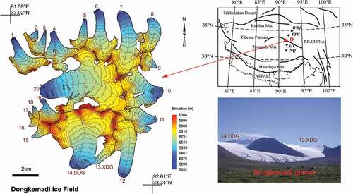
Figure 2. Comparison of (a) the reconstructed and observed daily air temperatures from 1991 to 1994 and (b) the monthly precipitation and observed from 1 July 2005 to 12 December 2008. The observed daily air temperature are from Fujita et al. (2000) and monthly precipitation is from H. Gao, He, et al. (2012)

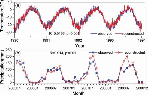
Figure 3. (a) Extrapolated daily mean air temperature and precipitation at the terminus of the XDG from 1989 to 2012 and downscaled daily mean air temperature and precipitation for (b) RCP 4.5 and (c) RCP 8.5, respectively

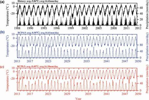
Table 1. Ground-based meteorological data

Stations	Periods	Latitude (° N)	Longitude (° E)	Altitude (m a.s.l.)	Pannual (mm)	Psummer (mm)	Tannual (°C)	Tsummer (°C)
WDL	1957–2013	35.22	93.08	4,612	278.1	256.0	−5.37	2.94
TTH	1957–2013	34.22	92.43	4,533	280.9	259.1	−4.05	4.96
AD	1966–2013	32.35	91.10	4,800	442.2	404.5	−2.80	5.62
NQ	1955–2013	31.48	92.07	4,507	398.7	353.8	−1.28	6.85

Notes. P_annual and P_summer denote annual and summer precipitation, respectively, and T_annual and T_summer indicate annual and summer air temperatures, respectively. WDL, TTH, AD, and NQ indicate the Wudaoliang, Tuotuohe, Anduo and Naqu weather stations, respectively.

Table 2. Applied parameters of the model optimized for all measured mass balance series in the DIF

Parameter	Value	Unit
Temperature lapse rate, λT	0.63	°C/(100 m)
Melt factor, fm	4	mm day^−1°C^−1
Radiation coefficient for snow, αsnow	7.5	mm day^−1 W^−1 m^2°C^−1
Radiation coefficient for ice,αice	15	mm day^−1 W^−1 m^2°C^−1
Precipitation gradient, λP	30	%/100 m
Precipitation correction factor, S	25	%

Figure 4. Comparison between simulated and measured (a) annual mass balance and (b) ELA and (c) scatterplot of calculated vs. measured mass balance at individual stakes on the XDG. The vertical bar denotes the 1δ standard deviation

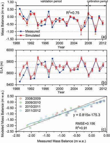
Figure 5. Seasonal variation in mass balance in the DIF during the period 1989 to 2050 under RCP 4.5 and RCP 8.5. The blue and red bars denote accumulation and ablation, respectively, and the black samples and line refer to the annual net mass balance. Error bar indicates the standard deviation of the results

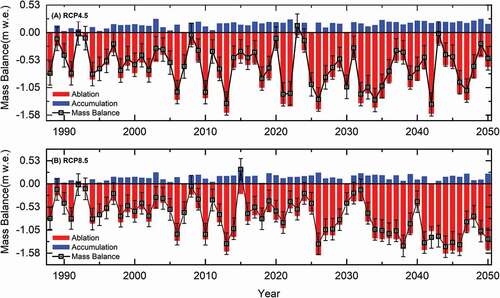
Table 3. The annual mean mass balance of the XDG and DIF during different periods

	Glaciological results^a	Geodetic results^b		Simulated results^c
Period	XDG (m w.e. year^−1)	XDG (m w.e. year^−1)	DIF (m w.e. year^−1)	XDG (m w.e. year^−1)	DIF (m w.e. year^−1)
1969–1999	—	−0.06 ± 0.10	–0.21 ± 0.10	—	—
1989–1999	−0.12	—	—	−0.14	−0.46
1999–2015	−0.42	−0.41 ± 0.21	–0.74 ± 0.21	−0.39 ± 0.01	−0.56 ± 0.01
2015–2050	—	—	—	−0.63 ± 0.07	−0.72 ± 0.07
1989–2050	—	—	—	−0.48 ± 0.05	−0.64 ± 0.05

Notes. ^aData from Pu et al. (2007).

^bData from Chen et al. (2017).

^cThis study.

Figure 6. (a) Accumulated mass balance during 1989 to 2050 and (b) anomalies in accumulated annual mass balance

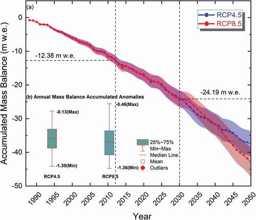
Figure 7. (a) Distribution of area and (b) mass balance from 1989 to 2012 in (c) RCP 4.5 and (d) RCP 8.5 with respect to altitude in the DIF

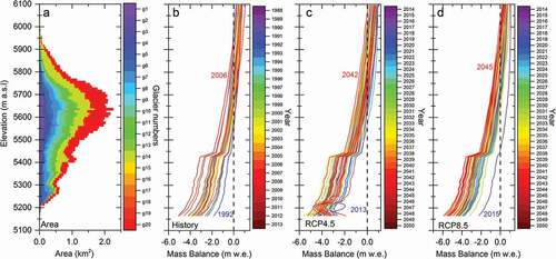
Figure 8. Variation in each individual glacier in the DIF from 1989 through future scenarios for 2050

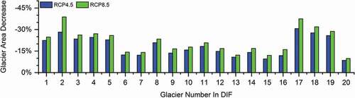
Figure 9. (a) Total area decrease and (b) volume of accumulated loss from 1989 to 2050 in the DIF. The shaded area indicates the 1δ deviation in the data

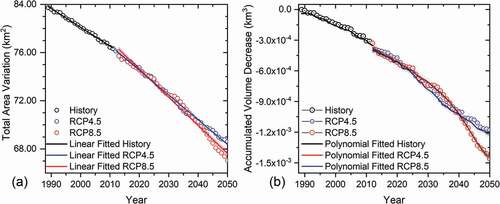
Figure 10. Spatial variation in mass balance and terminus elevation of the (a) DDG and (b) XDG from 1989 to 2012. The black lines show the glacier boundaries in 1989 and the red numbers are the altitudes of the glacier terminus in the respective years

Figure 11. Spatial variation in mass balance and terminus elevation for all glaciers in the DIF from 1989 to 2050. The black lines show the glacier boundaries in 1989

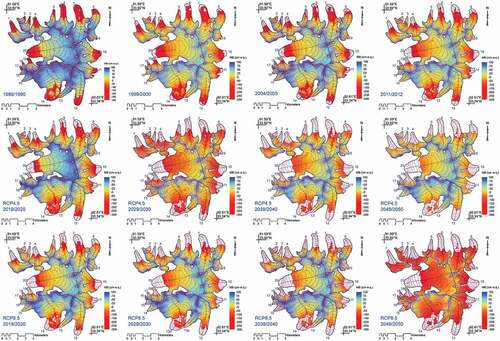
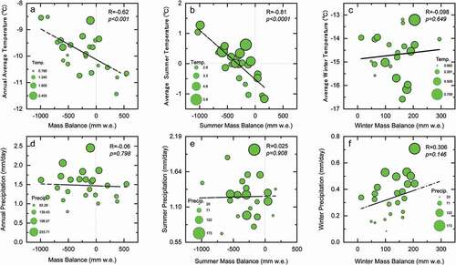
Figure 12. Correlation between mass balance and means (annual, summer, and winter air temperatures) or total (annual, summer, and winter precipitation) local climate forcing from simple linear regression analysis for 1989 to 2012 in the XDG. Dashed lines represent changing trends with indicators. The summer season corresponds to the months June to September

Fujita, K., Y. Ageta, P. Jianchen, and Y. Tandong. 2000. Mass balance of Xiao Dongkemadi glacier on the central Tibetan Plateau from 1989 to 1995. Annals of Glaciology 31 (1):159–63. doi:https://doi.org/10.3189/172756400781820075.

 Google Scholar

Gao, H., X. He, B. Ye, and J. Pu. 2012. Modeling the runoff and glacier mass balance in a small watershed on the Central Tibetan Plateau, China, from 1955 to 2008. Hydrological Processes 26 (11):1593–603. doi:https://doi.org/10.1002/hyp.v26.11.

 Web of Science ®Google Scholar

Chen, A., N. Wang, Z. Li, Y. Wu, W. Zhang, and Z. Guo. 2017. Region-wide glacier mass budgets for the Tanggula Mountains between ~1969 and ~2015 derived from remote sensing data. Arctic, Antarctic, and Alpine Research 49 (4):551–68. doi:https://doi.org/10.1657/AAAR0016-065.

 Web of Science ®Google Scholar