Figures & data
Figure 1. Study area, including Alaska and Eastern Siberia, as well as the hydrometeorological stations used to assess the hydrodynamic and wave modeling approach.
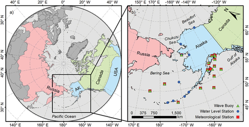
Figure 2. (a) Developed numerical mesh, with higher resolution in the (b) coast of Alaska. Mesh resolution is given by the distance between nodes in kilometers.
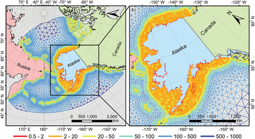
Table 1. Available wind and pressure forcing products implemented in the proposed ADCIRC+SWAN model
Figure 3. Storm progression in terms of wind magnitude and speed and MSL pressure during (a) Storm 1, (b) Storm 2, and (c) Storm 3.
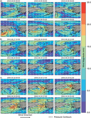
Figure 4. Observed and simulated storm surges (total water level − tides) for all available wind and pressure forcings during Storm 1.
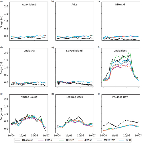
Figure 5. Observed and simulated storm surges (total water level − tides) for all available wind and pressure forcings during Storm 2.
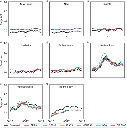
Figure 6. Observed and simulated storm surges (total water level − tides) for all available wind and pressure forcings during Storm 3.
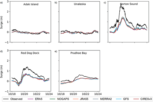
Figure 7. Observed and simulated Hs for all available wind and pressure forcings during Storm 1.
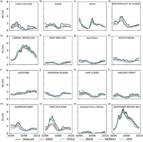
Figure 8. Observed and simulated Hs for all available wind and pressure forcings during Storm 2.
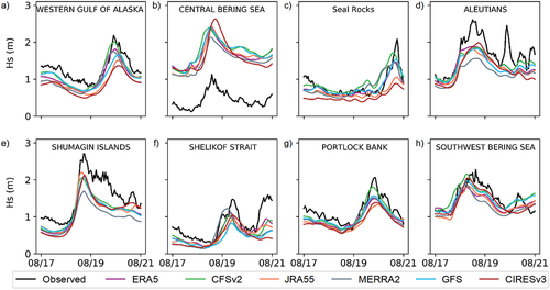
Figure 9. Observed and simulated Hs for all available wind and pressure forcings during Storm 3.
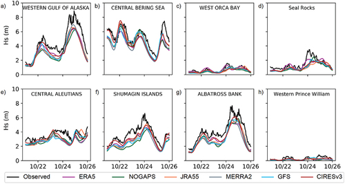
Figure 10. Taylor diagram of (a)–(c) surges and (d)–(f) waves for individual stations (small “x”) as well as averaged by storm (large “x”). The blue triangle indicates the observed data.
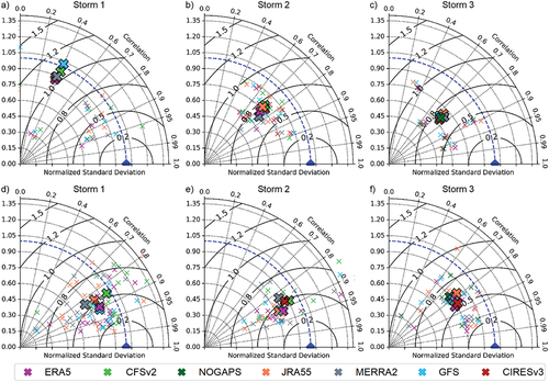
Table 2. Storm surge RMSE (in meters) for each station and storm for all forcings considered
Table 3. Hs RMSE (in meters) for each buoy and storm for all forcings considered
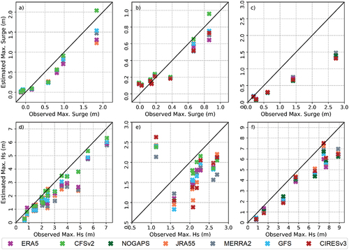
Figure 11. Peak (a)–(c) surge and (d)–(f) Hs for each monitored station during (a), (d) Storm 1, (b), (e) Storm 2, and (c), (f) Storm 3.